DeTime Method Gallery

This gallery follows the same pattern as a Sphinx-Gallery example page: short explanation, executable code blocks, printed output, figures, and download links. The examples use compact synthetic data so they run quickly in docs builds and local checkouts.

Regenerate this page and its assets with python scripts/generate_notebook_gallery.py.

Animated method explanations show the calculation steps for every registered method, with GIFs, static images and source arrays.

Imports and synthetic data

import sys
import warnings
from pathlib import Path

import matplotlib.pyplot as plt
import numpy as np
import pandas as pd
from IPython.display import display

# Prefer the checkout when this notebook is run inside the repository.
repo_src = Path.cwd() / "src"
if (repo_src / "detime").exists():
    sys.meta_path[:] = [
        finder for finder in sys.meta_path
        if not any(token in finder.__class__.__module__.lower() for token in ("detime", "de_time"))
    ]
    sys.path.insert(0, str(repo_src))

from detime import DecompositionConfig, MethodRegistry, decompose

warnings.filterwarnings("ignore", category=FutureWarning)
plt.rcParams.update(
    {
        "figure.figsize": (7.6, 3.0),
        "figure.dpi": 130,
        "savefig.dpi": 220,
        "axes.grid": False,
        "axes.spines.top": False,
        "axes.spines.right": False,
        "font.size": 10,
    }
)

rng = np.random.default_rng(42)
t = np.arange(96, dtype=float)
seasonal = np.sin(2.0 * np.pi * t / 12.0)
slow = 0.018 * t + 0.25 * np.sin(2.0 * np.pi * t / 48.0)
noise = 0.05 * rng.standard_normal(t.shape)
series = slow + seasonal + noise
panel = np.column_stack(
    [
        series,
        0.8 * slow + np.sin(2.0 * np.pi * (t + 2.0) / 12.0) + 0.04 * rng.standard_normal(t.shape),
        1.15 * slow + 0.7 * np.sin(2.0 * np.pi * (t + 4.0) / 12.0) + 0.04 * rng.standard_normal(t.shape),
    ]
)

CASES = {
    "SSA": {"data": series, "config": {"method": "SSA", "params": {"window": 24, "rank": 6, "primary_period": 12}, "backend": "auto", "speed_mode": "exact"}},
    "STD": {"data": series, "config": {"method": "STD", "params": {"period": 12}, "backend": "auto"}},
    "STDR": {"data": series, "config": {"method": "STDR", "params": {"period": 12}, "backend": "auto"}},
    "MSSA": {"data": panel, "config": {"method": "MSSA", "params": {"window": 24, "rank": 6, "primary_period": 12}, "backend": "python", "channel_names": ["a", "b", "c"]}},
    "STL": {"data": series, "config": {"method": "STL", "params": {"period": 12}}},
    "MSTL": {"data": series, "config": {"method": "MSTL", "params": {"periods": [12, 24]}}},
    "ROBUST_STL": {"data": series, "config": {"method": "ROBUST_STL", "params": {"period": 12}}},
    "EMD": {"data": series, "config": {"method": "EMD", "params": {"primary_period": 12, "n_imfs": 4}}},
    "CEEMDAN": {"data": series, "config": {"method": "CEEMDAN", "params": {"primary_period": 12, "trials": 3, "noise_width": 0.03}}},
    "VMD": {"data": series, "config": {"method": "VMD", "params": {"K": 4, "alpha": 300.0, "primary_period": 12}}},
    "WAVELET": {"data": series, "config": {"method": "WAVELET", "params": {"wavelet": "db4", "level": 3}}},
    "MA_BASELINE": {"data": series, "config": {"method": "MA_BASELINE", "params": {"trend_window": 7, "season_period": 12}}},
    "MVMD": {"data": panel, "config": {"method": "MVMD", "params": {"K": 4, "alpha": 300.0, "primary_period": 12}, "channel_names": ["a", "b", "c"]}},
    "MEMD": {"data": panel, "config": {"method": "MEMD", "params": {"primary_period": 12}, "channel_names": ["a", "b", "c"]}},
    "GABOR_CLUSTER": {"data": series, "skip": "requires a trained GaborClusterModel or model_path plus the experimental clustering backend"},
}

GALLERY_RESULTS = []

def _plot_vector(values):
    arr = np.asarray(values, dtype=float)
    if arr.ndim == 2:
        return arr[:, 0]
    return arr


def _style_gallery_axis(ax, title):
    ax.set_facecolor("#ffffff")
    ax.grid(True, axis="y", alpha=0.22, color="#94a3b8", linewidth=0.8)
    ax.grid(False, axis="x")
    ax.spines["left"].set_color("#cbd5e1")
    ax.spines["bottom"].set_color("#cbd5e1")
    ax.tick_params(colors="#334155")
    ax.set_title(title, loc="left", fontsize=12, fontweight="bold", color="#0f172a")


def run_gallery_case(name):
    case = CASES[name]
    metadata = MethodRegistry.get_metadata(name)
    print(f"{name}: {metadata['summary']}")
    if "skip" in case:
        row = {
            "method": name,
            "status": "skipped",
            "reason": case["skip"],
            "input_mode": metadata["input_mode"],
            "output_shape": "",
            "reconstruction_rmse": np.nan,
        }
        GALLERY_RESULTS.append(row)
        display(pd.DataFrame([row]))
        return

    data = case["data"]
    cfg = DecompositionConfig(**case["config"])
    try:
        result = decompose(data, cfg)
    except Exception as exc:
        row = {
            "method": name,
            "status": "skipped",
            "reason": f"{type(exc).__name__}: {exc}",
            "input_mode": metadata["input_mode"],
            "output_shape": "",
            "reconstruction_rmse": np.nan,
        }
        GALLERY_RESULTS.append(row)
        display(pd.DataFrame([row]))
        return

    original = _plot_vector(data)
    trend = _plot_vector(result.trend)
    season = _plot_vector(result.season)
    residual = _plot_vector(result.residual)
    reconstruction = np.asarray(result.trend) + np.asarray(result.season) + np.asarray(result.residual)
    rmse = float(np.sqrt(np.mean((np.asarray(data) - reconstruction) ** 2)))

    row = {
        "method": name,
        "status": "ran",
        "reason": "",
        "input_mode": metadata["input_mode"],
        "output_shape": str(np.asarray(result.trend).shape),
        "reconstruction_rmse": round(rmse, 8),
    }
    GALLERY_RESULTS.append(row)
    display(pd.DataFrame([row]))

    fig, ax = plt.subplots(facecolor="#f8fafc")
    ax.plot(original, label="input", color="#0f172a", linewidth=1.6)
    ax.plot(trend, label="trend", color="#2563eb", linewidth=1.4)
    ax.plot(season, label="season", color="#0f766e", linewidth=1.2)
    ax.plot(residual, label="residual", color="#f97316", linewidth=1.0, alpha=0.85)
    _style_gallery_axis(ax, f"{name} decomposition")
    ax.set_xlabel("time step")
    ax.legend(loc="upper right", ncol=2, fontsize=8, frameon=True, framealpha=0.92)
    fig.tight_layout()
    plt.show()

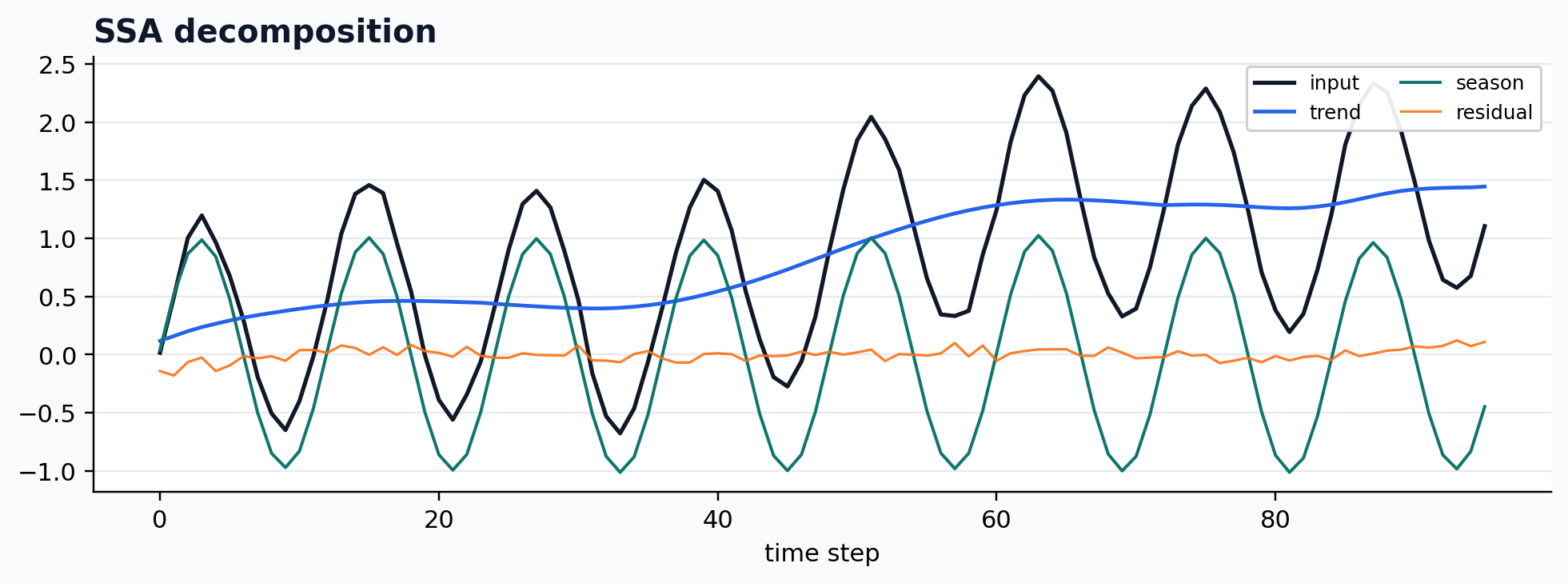
Univariate SSA

Watch how SSA works.

case = CASES["SSA"]
run_gallery_case("SSA")

Out:

SSA: Singular spectrum analysis for structured univariate decomposition.
status: ran
input mode: univariate
trend shape: (96,)
backend: native
reconstruction RMSE: 0.00000000

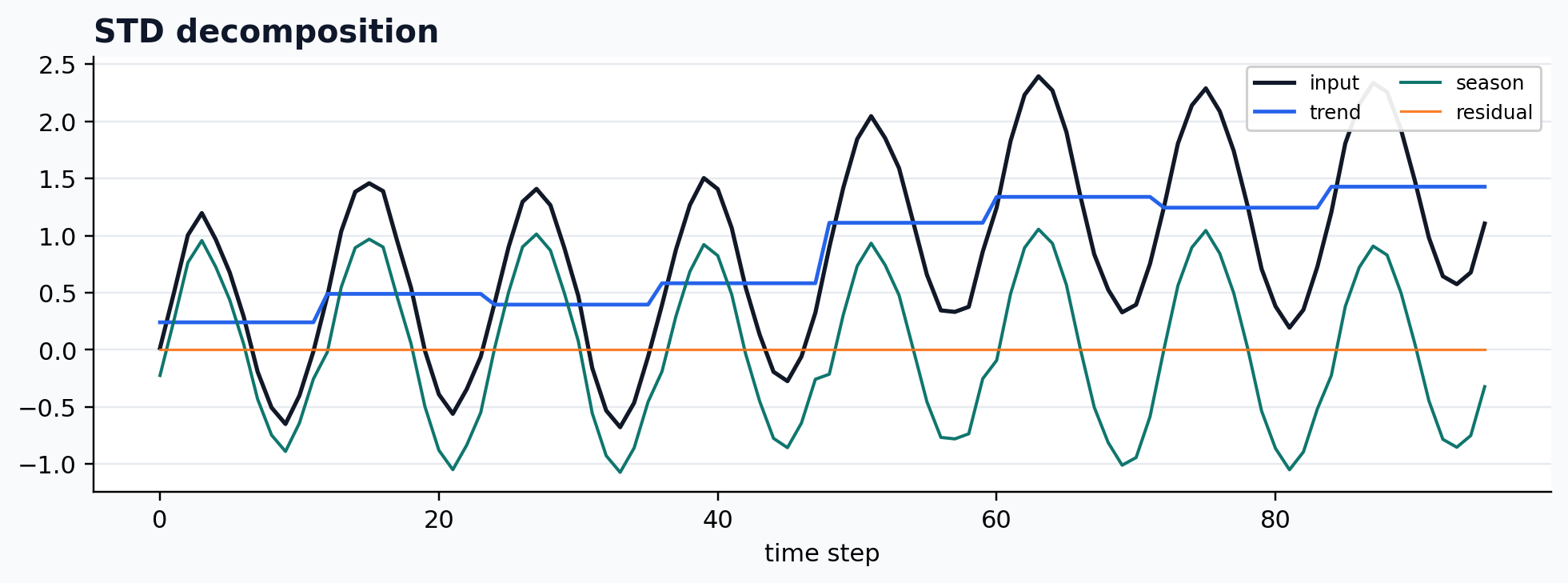
Seasonal-trend-dispersion decomposition

Watch how STD works.

case = CASES["STD"]
run_gallery_case("STD")

Out:

STD: Fast seasonal-trend decomposition with dispersion-aware diagnostics.
status: ran
input mode: channelwise
trend shape: (96,)
backend: native
reconstruction RMSE: 0.00000000

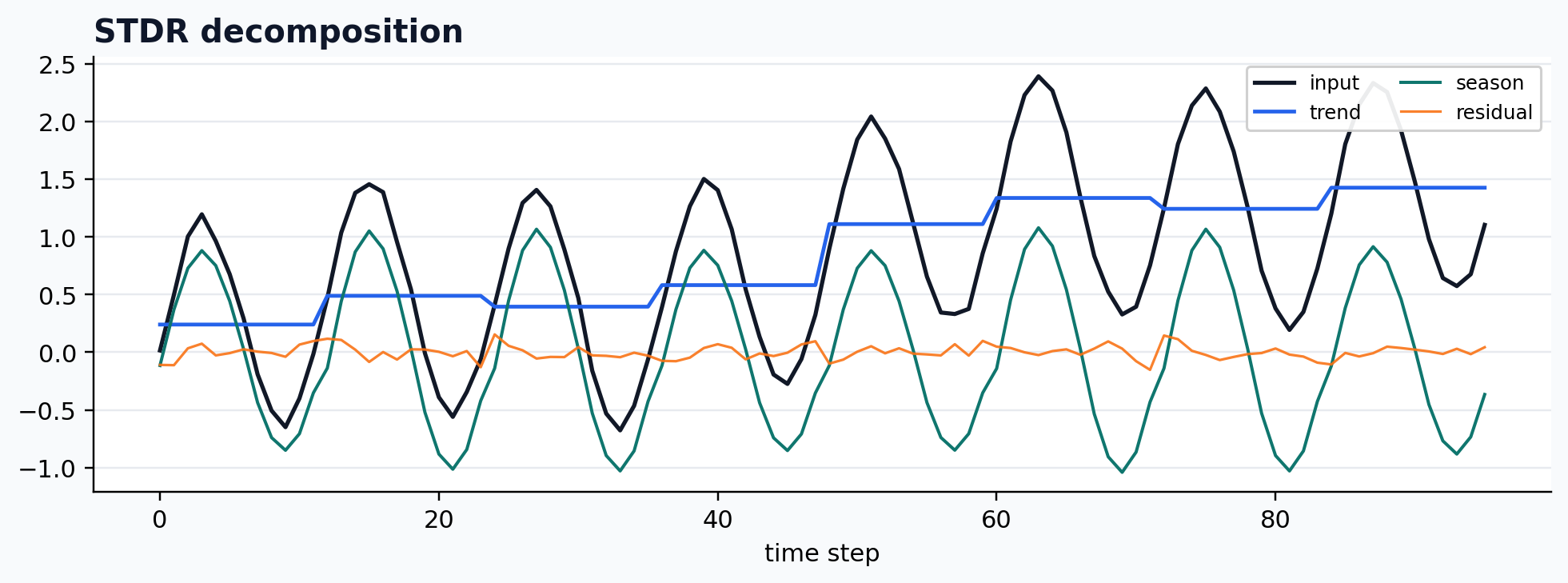
Seasonal-trend-dispersion decomposition with a remainder

Watch how STDR works.

case = CASES["STDR"]
run_gallery_case("STDR")

Out:

STDR: Seasonal-trend-dispersion decomposition with an averaged cycle shape and a remainder.
status: ran
input mode: channelwise
trend shape: (96,)
backend: native
reconstruction RMSE: 0.00000000

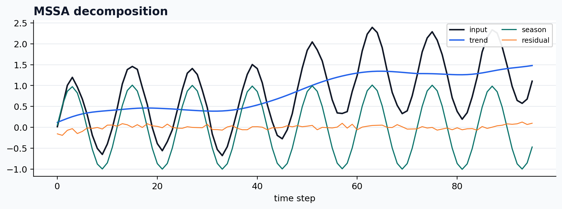
Multivariate SSA

Watch how MSSA works.

case = CASES["MSSA"]
run_gallery_case("MSSA")

Out:

MSSA: Multivariate SSA for shared-structure decomposition across channels.
status: ran
input mode: multivariate
trend shape: (96, 3)
backend: python
reconstruction RMSE: 0.00000000

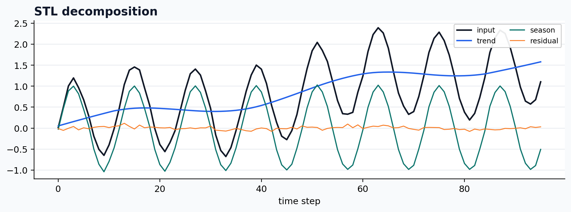
Statsmodels STL wrapper

Watch how STL works.

case = CASES["STL"]
run_gallery_case("STL")

Out:

STL: Classical STL wrapped into the DeTime workflow contract.
status: ran
input mode: univariate
trend shape: (96,)
backend: python
reconstruction RMSE: 0.00000000

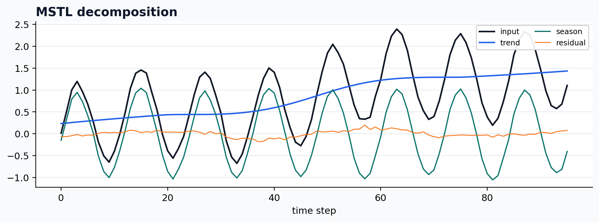
Statsmodels MSTL wrapper

Watch how MSTL works.

case = CASES["MSTL"]
run_gallery_case("MSTL")

Out:

MSTL: Statsmodels MSTL wrapped into the DeTime workflow surface.
status: ran
input mode: univariate
trend shape: (96,)
backend: python
reconstruction RMSE: 0.00000000

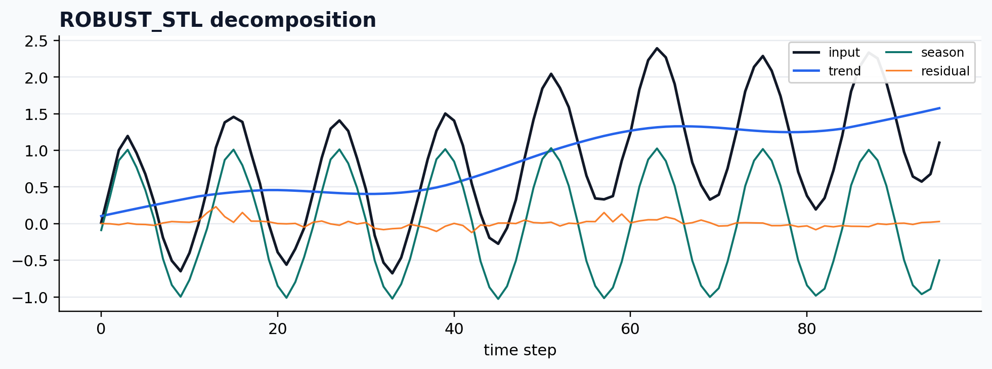
Robust STL wrapper

Watch how ROBUST_STL works.

case = CASES["ROBUST_STL"]
run_gallery_case("ROBUST_STL")

Out:

ROBUST_STL: Robust STL-style decomposition wrapped for reproducible workflows.
status: ran
input mode: univariate
trend shape: (96,)
backend: python
reconstruction RMSE: 0.00000000

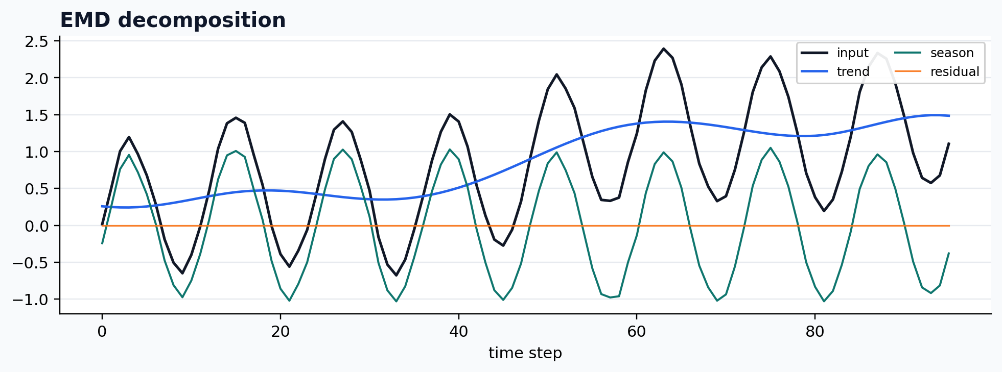
Empirical mode decomposition

Watch how EMD works.

case = CASES["EMD"]
run_gallery_case("EMD")

Out:

EMD: Empirical mode decomposition under the DeTime result contract.
status: ran
input mode: univariate
trend shape: (96,)
backend: python
reconstruction RMSE: 0.00000000

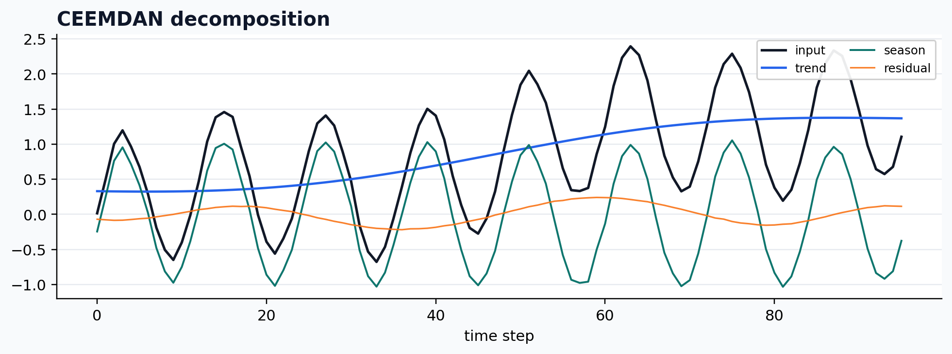
Noise-assisted EMD

Watch how CEEMDAN works.

case = CASES["CEEMDAN"]
run_gallery_case("CEEMDAN")

Out:

CEEMDAN: Noise-assisted EMD wrapper with IMFs in (mode, time, channel) layout.
status: ran
input mode: univariate
trend shape: (96,)
backend: python
reconstruction RMSE: 0.00000000

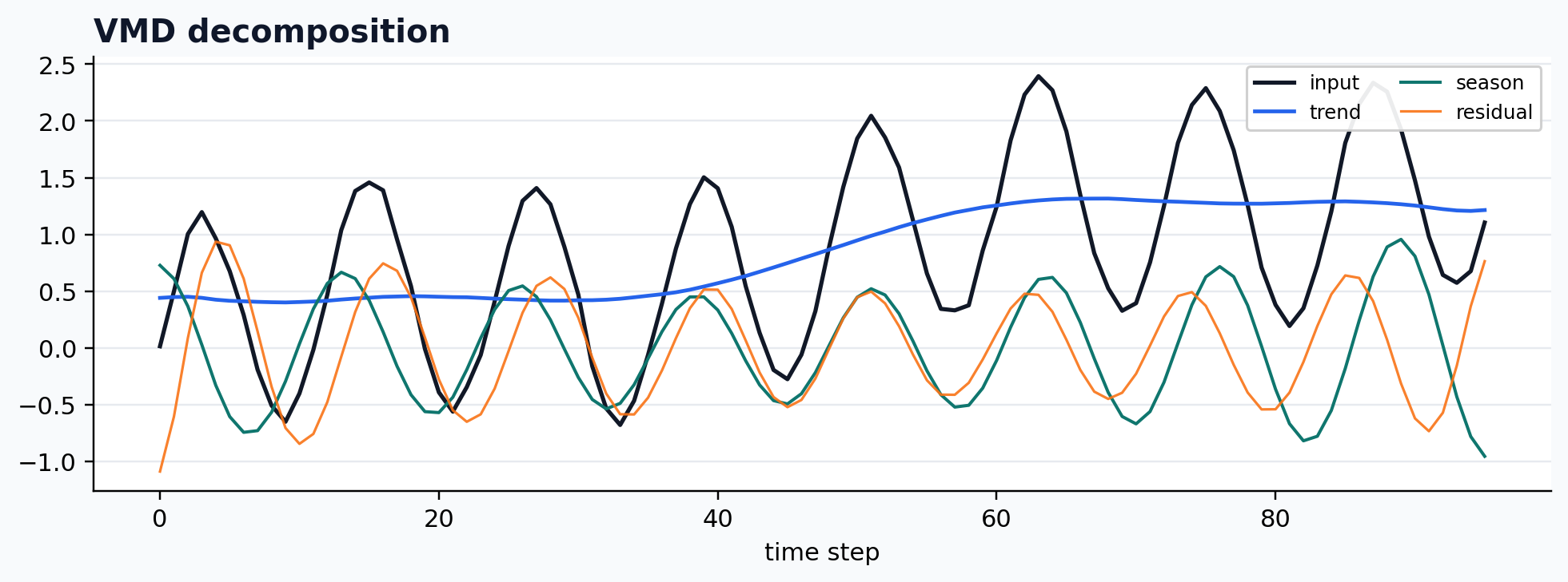
Variational mode decomposition

Watch how VMD works.

case = CASES["VMD"]
run_gallery_case("VMD")

Out:

VMD: Variational mode decomposition integrated into the common workflow layer.
status: ran
input mode: univariate
trend shape: (96,)
backend: native
reconstruction RMSE: 0.00000000

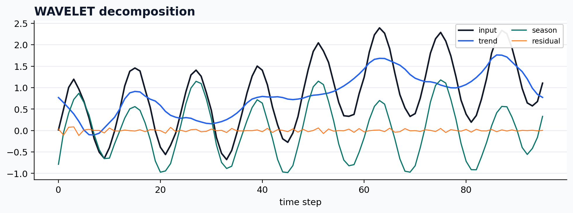
Wavelet decomposition

Watch how WAVELET works.

case = CASES["WAVELET"]
run_gallery_case("WAVELET")

Out:

WAVELET: Wavelet-based decomposition exposed through the common output contract.
status: ran
input mode: univariate
trend shape: (96,)
backend: python
reconstruction RMSE: 0.00000000

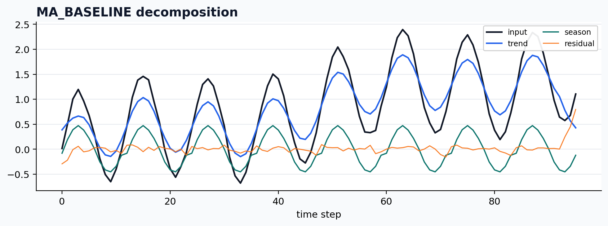
Moving-average baseline

Watch how MA_BASELINE works.

case = CASES["MA_BASELINE"]
run_gallery_case("MA_BASELINE")

Out:

MA_BASELINE: Simple moving-average baseline for smoke tests and lightweight workflows.
status: ran
input mode: univariate
trend shape: (96,)
backend: native
reconstruction RMSE: 0.00000000

Optional multivariate VMD backend

Watch how MVMD works.

case = CASES["MVMD"]
run_gallery_case("MVMD")

Out:

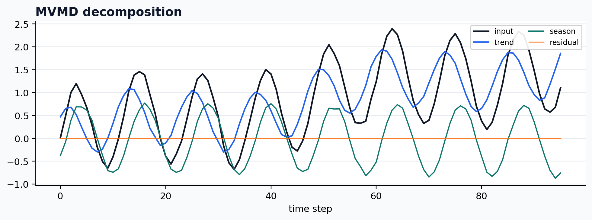
MVMD: Optional multivariate VMD backend for shared frequency structure.
status: ran
input mode: multivariate
trend shape: (96, 3)
backend: python
reconstruction RMSE: 0.00000000

Optional multivariate EMD backend

Watch how MEMD works.

case = CASES["MEMD"]
run_gallery_case("MEMD")

Out:

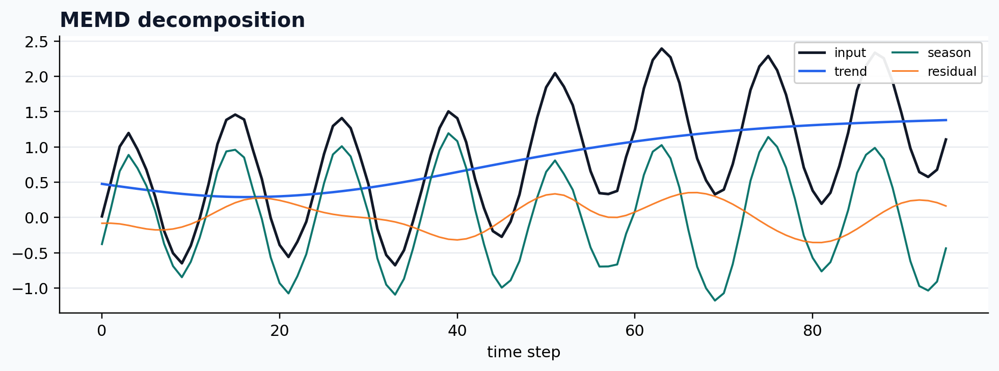
MEMD: Optional multivariate EMD backend for shared oscillatory structure.
status: ran
input mode: multivariate
trend shape: (96, 3)
backend: python
reconstruction RMSE: 0.00000000

Experimental Gabor clustering path

Watch how GABOR_CLUSTER works.

case = CASES["GABOR_CLUSTER"]
print(case["skip"])

Out:

requires a trained GaborClusterModel or model_path plus the experimental clustering backend

Summary

Reconstruction RMSE is computed from input minus the sum of trend, season, and residual over all samples and channels. It checks additive bookkeeping, not forecasting accuracy or recovery of ground-truth components.

Total running time of the gallery script: 4.746 seconds.

Methods run: 14; skipped with explicit reason: 1.

Downloads

The GitHub-rendered notebook is also available at examples/notebooks/de_time_method_gallery.ipynb.