Robust STL wrapper
Robust STL wrapper
| Property | Value |
|---|---|
| Method | ROBUST_STL |
| Input mode | univariate |
| Trend shape | (96,) |
| Notebook execution | ran |
| Reconstruction RMSE | 0.00000000 |
Notebook example metric: root mean square of input - (trend + season + residual) over all samples and channels. This checks additive bookkeeping; it is not a forecast error or a component-recovery score. The separate teaching input and intermediate arrays for the animation are linked below.
How it works
Method maturity: stable. Implementation: wrapper.
Residual-based robustness weights limit how strongly unusual observations influence subsequent STL smooths.
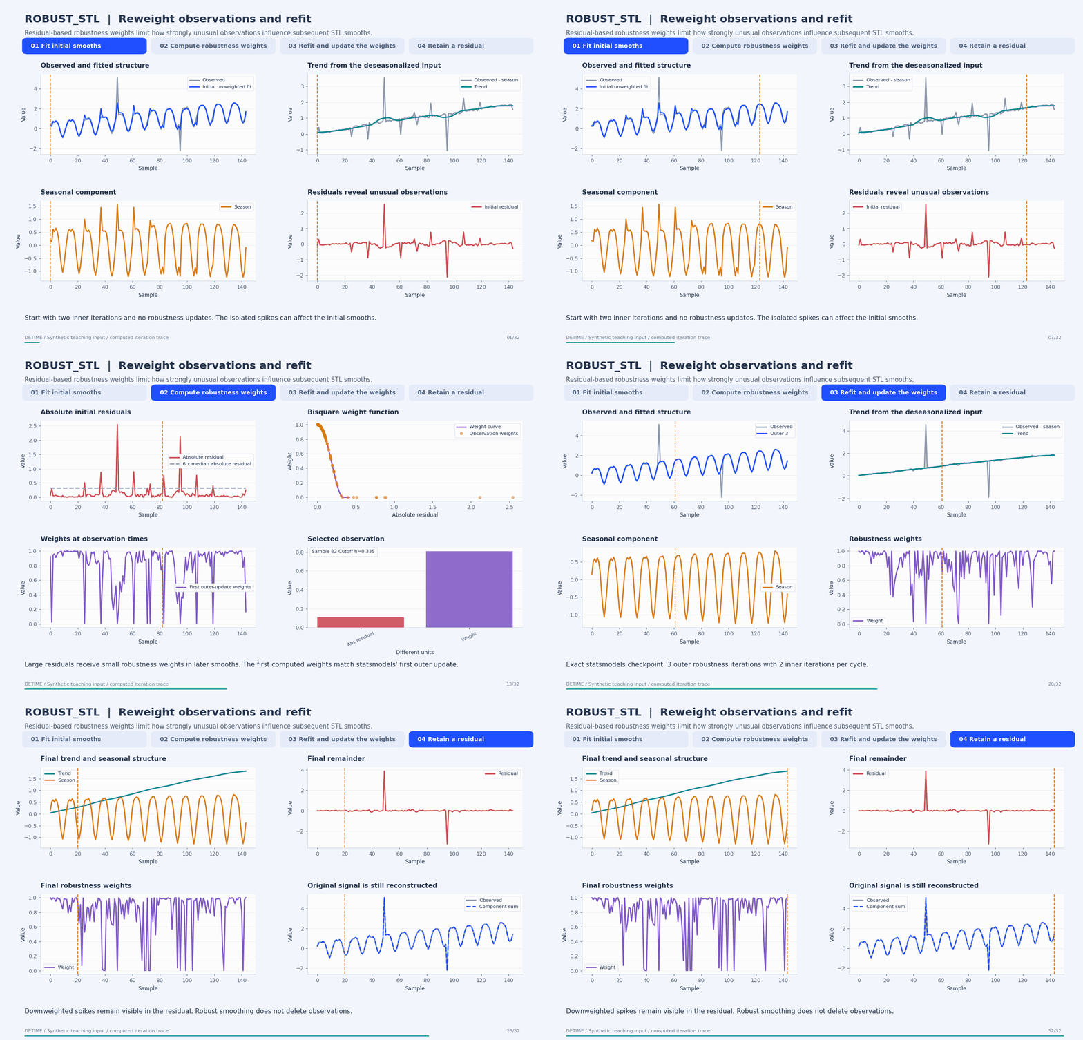
Deterministic synthetic teaching signal; not a benchmark.
Open GIF · Static PNG · Source arrays (NPZ) · Trace metadata
Follow the four steps
1. Fit initial smooths
DeTime's ROBUST_STL selects statsmodels STL with robust=True by default. The initial inner loop estimates seasonal and trend structure before robustness weights are updated.
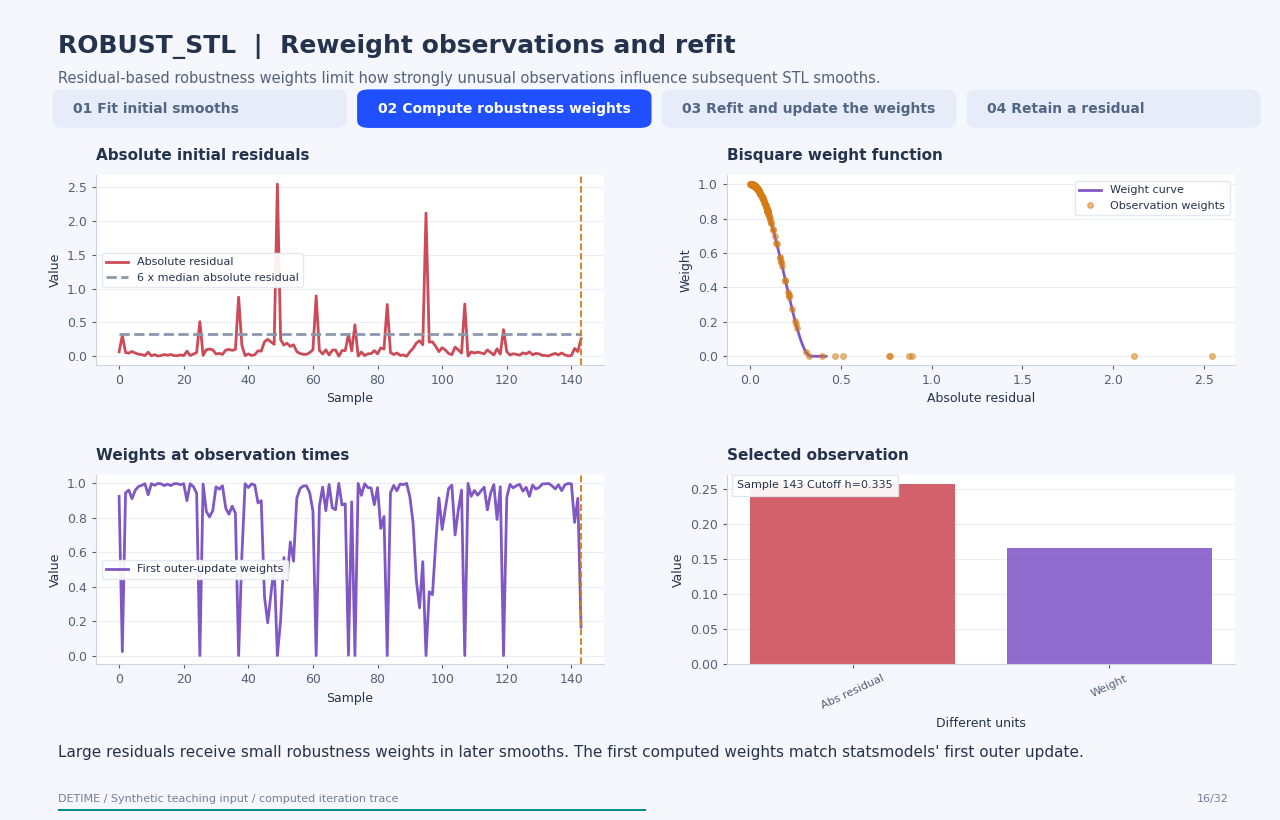
2. Compute robustness weights
The first outer update uses absolute residuals from the initial fit. With h equal to six times their median, the bisquare rule assigns (1 - (abs(residual)/h)^2)^2 below h and zero above h. This example computes those weights and checks them against statsmodels.
3. Refit and update the weights
Repeated outer iterations recalculate robustness weights and refit seasonal and trend smooths. Each shown checkpoint is a fresh deterministic statsmodels fit with the indicated iteration budget; it reaches the same state for that budget.
4. Retain a residual
The wrapper returns the final trend, seasonal component, and residual. Downweighted observations remain in the input, so their unexplained values appear in the residual. The animation also displays upstream weights, which the current DeTime wrapper does not export as a result component.
Parameters that change the result
| Parameter | Effect on the computation |
|---|---|
period |
Specified number of samples in a seasonal cycle; this example uses 12. |
seasonal |
Odd LOESS span across cycles for the seasonal subseries; smaller spans allow faster seasonal change. |
trend / low_pass |
Odd smoothing spans controlling trend and low-pass behavior; this example uses 23 and 13. |
robust |
Controls the outer reweighting loop. ROBUST_STL defaults to True; setting it False disables robustness. |
What this animation computes
All robustness weights and iteration checkpoints are computed from statsmodels; the first bisquare update is independently calculated and compared. Final arrays match DeTime's Python wrapper.
Interpretation
- ROBUST_STL is the registry name for statsmodels STL with its robust option. This name does not establish implementation of other published algorithms also called RobustSTL.
- Smoothing spans, seasonal period, endpoint handling, and outliers influence the estimated components.
- The animation uses statsmodels' actual checkpoints. Internal fits are restarted for each budget; frame count is not an execution-time measure.
- STL is an offline smoother. Use only available history when constructing forecasting features.
Try the method
Use this configuration with DecompositionConfig and decompose. The animation generator supplies the teaching input and records intermediate arrays.
{
  "method": "ROBUST_STL",
  "backend": "python",
  "params": {
    "period": 12,
    "seasonal": 7,
    "trend": 23,
    "low_pass": 13,
    "robust": true
  }
}
See the configuration reference for the full interface and optional dependencies.
Sources and reproduction
- Cleveland et al. (1990), STL: A Seasonal-Trend Decomposition Procedure Based on Loess
- statsmodels STL: parameters and implementation contract
- DeTime implementation:
src/detime/methods/stl.py
Regenerate this animation with python scripts/generate_method_animations.py --methods ROBUST_STL.
The reproduction guide explains the environment,
numerical checks, coverage manifest, and how to inspect the stored arrays.
Code
case = CASES["ROBUST_STL"]
run_gallery_case("ROBUST_STL")
Output
ROBUST_STL: Robust STL-style decomposition wrapped for reproducible workflows.
status: ran
input mode: univariate
trend shape: (96,)
backend: python
reconstruction RMSE: 0.00000000
Decomposition Plot
