AI Infrastructure Market Pulse
Executed Notebook
This notebook asks how a defined AI-infrastructure market-price basket moved over the selected window. The basket is a public price proxy for attention around compute, cloud, chips, platforms, and adjacent high-interest names.
The output is a basket definition, a source card, trend-index figures, return-versus-trend comparison, and edge-trimmed residual events. Revenue, capex, margins, and valuation require official financial data.
In [1]
from pathlib import Path
import os

import matplotlib.pyplot as plt
import numpy as np
import pandas as pd

from examples.hot_trends.data import (
    HotTrendDataError,
    append_real_snapshot,
    build_arxiv_monthly_counts,
    fetch_coingecko_market_chart,
    fetch_defillama_stablecoin_chains,
    fetch_github_repo_metadata,
    fetch_github_stargazers,
    fetch_huggingface_models,
    fetch_wikipedia_pageviews,
    source_audit_table,
)
from examples.hot_trends.decomposition import (
    component_summary,
    decompose_table,
    editorial_priority,
    residual_event_table,
)
from examples.hot_trends.scoring import article_publication_phrasing

pd.set_option("display.max_columns", 80)
pd.set_option("display.max_rows", 80)
plt.rcParams.update({"axes.grid": True})

CACHE_DIR = Path("examples/hot_trends/cache")
OUTPUT_DIR = Path("examples/hot_trends/outputs")
CACHE_DIR.mkdir(parents=True, exist_ok=True)
OUTPUT_DIR.mkdir(parents=True, exist_ok=True)

def save_table(df, name):
    path = OUTPUT_DIR / f"{name}.csv"
    df.to_csv(path, index=False)
    print(f"saved: {path.as_posix()}")
1. Fetch prices through yfinance
In [2]
try:
    import yfinance as yf
except Exception as exc:
    raise ImportError("Install yfinance to run this notebook: python -m pip install yfinance") from exc

basket_definition = pd.DataFrame([
    {"ticker": "NVDA", "role": "GPU accelerator supplier", "boundary": "large-cap chip proxy, not pure infrastructure revenue"},
    {"ticker": "AMD", "role": "GPU/CPU accelerator challenger", "boundary": "mixed client, data-center, and gaming exposure"},
    {"ticker": "AVGO", "role": "networking and custom silicon", "boundary": "diversified semiconductor and software exposure"},
    {"ticker": "MSFT", "role": "cloud and AI platform", "boundary": "large diversified software/cloud company"},
    {"ticker": "GOOGL", "role": "cloud, TPU, and AI platform", "boundary": "advertising remains a major business line"},
    {"ticker": "AMZN", "role": "cloud infrastructure", "boundary": "retail and marketplace exposure included"},
    {"ticker": "META", "role": "AI compute demand and model deployment", "boundary": "advertising platform, not infrastructure vendor"},
    {"ticker": "TSLA", "role": "AI narrative and autonomous systems proxy", "boundary": "auto and energy exposure dominates fundamentals"},
])
tickers = basket_definition["ticker"].tolist()
start_date = "2024-01-01"
raw = yf.download(tickers, start=start_date, progress=False, auto_adjust=True)["Close"]
if raw.empty:
    raise HotTrendDataError("yfinance returned no market data")
prices = raw.reset_index().melt(id_vars="Date", var_name="ticker", value_name="price").rename(columns={"Date": "date"})
prices = prices.dropna(subset=["price"])
display(basket_definition)
prices.head(20)
text/html
|
ticker |
role |
boundary |
| 0 |
NVDA |
GPU accelerator supplier |
large-cap chip proxy, not pure infrastructure ... |
| 1 |
AMD |
GPU/CPU accelerator challenger |
mixed client, data-center, and gaming exposure |
| 2 |
AVGO |
networking and custom silicon |
diversified semiconductor and software exposure |
| 3 |
MSFT |
cloud and AI platform |
large diversified software/cloud company |
| 4 |
GOOGL |
cloud, TPU, and AI platform |
advertising remains a major business line |
| 5 |
AMZN |
cloud infrastructure |
retail and marketplace exposure included |
| 6 |
META |
AI compute demand and model deployment |
advertising platform, not infrastructure vendor |
| 7 |
TSLA |
AI narrative and autonomous systems proxy |
auto and energy exposure dominates fundamentals |
text/html
|
date |
ticker |
price |
| 0 |
2024-01-02 |
AMD |
138.580002 |
| 1 |
2024-01-03 |
AMD |
135.320007 |
| 2 |
2024-01-04 |
AMD |
136.009995 |
| 3 |
2024-01-05 |
AMD |
138.580002 |
| 4 |
2024-01-08 |
AMD |
146.179993 |
| 5 |
2024-01-09 |
AMD |
149.259995 |
| 6 |
2024-01-10 |
AMD |
148.539993 |
| 7 |
2024-01-11 |
AMD |
148.020004 |
| 8 |
2024-01-12 |
AMD |
146.559998 |
| 9 |
2024-01-16 |
AMD |
158.740005 |
| 10 |
2024-01-17 |
AMD |
160.169998 |
| 11 |
2024-01-18 |
AMD |
162.669998 |
| 12 |
2024-01-19 |
AMD |
174.229996 |
| 13 |
2024-01-22 |
AMD |
168.179993 |
| 14 |
2024-01-23 |
AMD |
168.419998 |
| 15 |
2024-01-24 |
AMD |
178.289993 |
| 16 |
2024-01-25 |
AMD |
180.330002 |
| 17 |
2024-01-26 |
AMD |
177.250000 |
| 18 |
2024-01-29 |
AMD |
177.830002 |
| 19 |
2024-01-30 |
AMD |
172.059998 |
2. Source card and price audit
In [3]
audit = source_audit_table(prices, value_col="price", entity_col="ticker", time_col="date")
source_card = pd.DataFrame([{
    "source": "Yahoo Finance through yfinance",
    "endpoint": "yfinance.download",
    "access_date": pd.Timestamp.today().date().isoformat(),
    "query_params": f"tickers={','.join(tickers)}; start={start_date}; auto_adjust=True; field=Close",
    "time_range": f"{pd.to_datetime(prices['date']).min().date()} to {pd.to_datetime(prices['date']).max().date()}",
    "cache_path": "not cached; outputs saved to examples/hot_trends/outputs",
    "interpretation_scope": "public market-price proxy for a defined basket; not fundamentals, valuation, or investment advice",
}])
display(source_card)
audit
text/html
|
source |
endpoint |
access_date |
query_params |
time_range |
cache_path |
interpretation_scope |
| 0 |
Yahoo Finance through yfinance |
yfinance.download |
2026-05-22 |
tickers=NVDA,AMD,AVGO,MSFT,GOOGL,AMZN,META,TSL... |
2024-01-02 to 2026-05-22 |
not cached; outputs saved to examples/hot_tren... |
public market-price proxy for a defined basket... |
text/html
|
series |
first_timestamp |
last_timestamp |
observations |
missing_ratio |
min_value |
max_value |
| 0 |
AMD |
2024-01-02 00:00:00 |
2026-05-22 00:00:00 |
600 |
0.0 |
78.209999 |
467.510010 |
| 1 |
AMZN |
2024-01-02 00:00:00 |
2026-05-22 00:00:00 |
600 |
0.0 |
144.570007 |
274.989990 |
| 2 |
AVGO |
2024-01-02 00:00:00 |
2026-05-22 00:00:00 |
600 |
0.0 |
102.365158 |
439.790009 |
| 3 |
GOOGL |
2024-01-02 00:00:00 |
2026-05-22 00:00:00 |
600 |
0.0 |
130.322876 |
402.619995 |
| 4 |
META |
2024-01-02 00:00:00 |
2026-05-22 00:00:00 |
600 |
0.0 |
341.787811 |
788.148987 |
| 5 |
MSFT |
2024-01-02 00:00:00 |
2026-05-22 00:00:00 |
600 |
0.0 |
351.105774 |
538.658508 |
| 6 |
NVDA |
2024-01-02 00:00:00 |
2026-05-22 00:00:00 |
600 |
0.0 |
47.539936 |
235.740005 |
| 7 |
TSLA |
2024-01-02 00:00:00 |
2026-05-22 00:00:00 |
600 |
0.0 |
142.050003 |
489.880005 |
3. Decompose normalized log prices
In [4]
components = decompose_table(prices, entity_col="ticker", time_col="date", value_col="price", method="MA_BASELINE", period=21, trend_window=63, transform="log")
summary = editorial_priority(component_summary(components, entity_col="ticker", time_col="date"), entity_col="ticker")
summary
text/html
|
ticker |
observations |
first_timestamp |
last_timestamp |
trend_last |
trend_slope_per_step |
cycle_strength_proxy |
residual_std |
max_abs_residual_z |
method |
trend_slope_per_step_rank_pct |
cycle_strength_proxy_rank_pct |
max_abs_residual_z_rank_pct |
editorial_priority_score |
| 2 |
AVGO |
600 |
2024-01-02 00:00:00 |
2026-05-22 00:00:00 |
3.056002 |
0.002033 |
-0.515611 |
0.492248 |
31.542094 |
MA_BASELINE |
1.000 |
1.000 |
0.500 |
0.77500 |
| 3 |
GOOGL |
600 |
2024-01-02 00:00:00 |
2026-05-22 00:00:00 |
2.996327 |
0.001351 |
-1.894425 |
0.500717 |
38.908369 |
MA_BASELINE |
0.625 |
0.500 |
1.000 |
0.76875 |
| 6 |
NVDA |
600 |
2024-01-02 00:00:00 |
2026-05-22 00:00:00 |
2.710889 |
0.001477 |
-0.730896 |
0.425016 |
30.472988 |
MA_BASELINE |
0.750 |
0.875 |
0.375 |
0.60625 |
| 7 |
TSLA |
600 |
2024-01-02 00:00:00 |
2026-05-22 00:00:00 |
3.037916 |
0.001532 |
-1.559972 |
0.528218 |
30.440903 |
MA_BASELINE |
0.875 |
0.750 |
0.250 |
0.56875 |
| 4 |
META |
600 |
2024-01-02 00:00:00 |
2026-05-22 00:00:00 |
3.277547 |
0.000695 |
-8.994860 |
0.545159 |
34.034109 |
MA_BASELINE |
0.500 |
0.375 |
0.625 |
0.53125 |
| 1 |
AMZN |
600 |
2024-01-02 00:00:00 |
2026-05-22 00:00:00 |
2.824287 |
0.000536 |
-12.700004 |
0.479970 |
38.328541 |
MA_BASELINE |
0.250 |
0.250 |
0.750 |
0.47500 |
| 5 |
MSFT |
600 |
2024-01-02 00:00:00 |
2026-05-22 00:00:00 |
3.058471 |
0.000199 |
-28.797940 |
0.536863 |
38.792840 |
MA_BASELINE |
0.125 |
0.125 |
0.875 |
0.46250 |
| 0 |
AMD |
600 |
2024-01-02 00:00:00 |
2026-05-22 00:00:00 |
2.973933 |
0.000667 |
-1.836756 |
0.521744 |
29.756925 |
MA_BASELINE |
0.375 |
0.625 |
0.125 |
0.31250 |
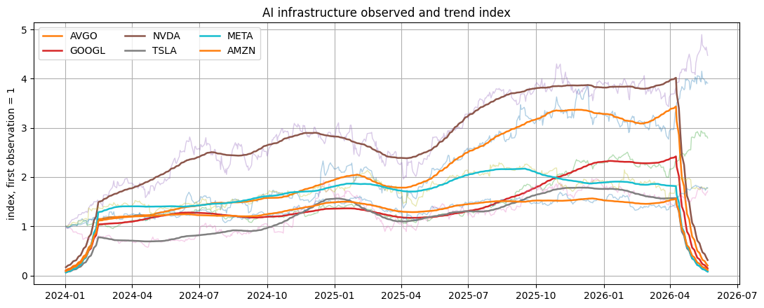
Visualization: AI infrastructure price trend index
The y-axis is an index with each ticker starting at 1. Solid trend lines make basket movement comparable across different share prices. This is a price-proxy view; benchmark and financial-statement evidence are needed before performance or valuation claims.
In [5]
top_tickers = summary["ticker"].head(6).tolist()
fig, ax = plt.subplots(figsize=(11, 4.5))
for ticker in top_tickers:
    panel = components.loc[components["ticker"].eq(ticker)].sort_values("date").copy()
    panel["date"] = pd.to_datetime(panel["date"])
    base = float(panel["observed"].iloc[0])
    observed_index = np.exp(panel["observed"] - base)
    trend_index = np.exp(panel["trend"] - base)
    ax.plot(panel["date"], observed_index, linewidth=1.0, alpha=0.35)
    ax.plot(panel["date"], trend_index, linewidth=1.8, label=ticker)
ax.set_title("AI infrastructure observed and trend index")
ax.set_ylabel("index, first observation = 1")
ax.legend(ncol=3, loc="best")
plt.tight_layout()
plt.show()
image/png
4. Cross-sectional AI infrastructure table
In [6]
latest = prices.sort_values("date").groupby("ticker").tail(1).rename(columns={"price": "latest_price"})
first = prices.sort_values("date").groupby("ticker").head(1).rename(columns={"price": "first_price"})[["ticker", "first_price"]]
returns = latest.merge(first, on="ticker", how="left")
returns["total_return_proxy"] = returns["latest_price"] / returns["first_price"] - 1.0
returns.sort_values("total_return_proxy", ascending=False)
text/html
|
date |
ticker |
latest_price |
first_price |
total_return_proxy |
| 6 |
2026-05-22 |
NVDA |
215.330002 |
48.138569 |
3.473128 |
| 3 |
2026-05-22 |
AVGO |
414.140015 |
105.914253 |
2.910144 |
| 5 |
2026-05-22 |
AMD |
467.510010 |
138.580002 |
2.373575 |
| 0 |
2026-05-22 |
GOOGL |
382.970001 |
137.037384 |
1.794639 |
| 4 |
2026-05-22 |
AMZN |
266.320007 |
149.929993 |
0.776296 |
| 2 |
2026-05-22 |
META |
610.260010 |
343.593658 |
0.776110 |
| 7 |
2026-05-22 |
TSLA |
426.010010 |
248.419998 |
0.714878 |
| 1 |
2026-05-22 |
MSFT |
418.570007 |
363.801514 |
0.150545 |
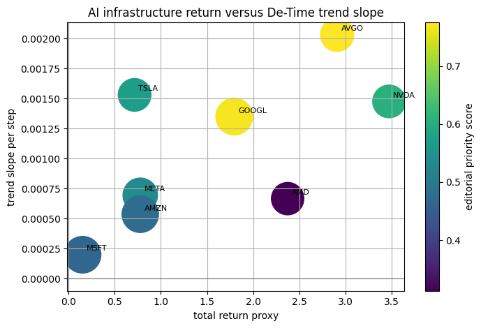
Visualization: return versus trend slope
The x-axis is simple total return over the sampled window. The y-axis is DeTime trend slope; marker size reflects residual shock magnitude. Read the scatter as a basket diagnostic, not as a recommendation.
In [7]
scatter_data = returns.merge(summary[["ticker", "trend_slope_per_step", "max_abs_residual_z", "editorial_priority_score"]], on="ticker", how="left")
fig, ax = plt.subplots(figsize=(7.2, 4.8))
sc = ax.scatter(
    scatter_data["total_return_proxy"],
    scatter_data["trend_slope_per_step"],
    s=80 + scatter_data["max_abs_residual_z"].fillna(0) * 35,
    c=scatter_data["editorial_priority_score"],
    cmap="viridis",
)
for _, row in scatter_data.iterrows():
    ax.annotate(str(row["ticker"]), (row["total_return_proxy"], row["trend_slope_per_step"]), fontsize=8, xytext=(4, 4), textcoords="offset points")
ax.axvline(0, color="0.45", linewidth=0.8)
ax.axhline(0, color="0.45", linewidth=0.8)
ax.set_xlabel("total return proxy")
ax.set_ylabel("trend slope per step")
ax.set_title("AI infrastructure return versus DeTime trend slope")
fig.colorbar(sc, ax=ax, label="editorial priority score")
plt.tight_layout()
plt.show()
image/png
5. Residual events
In [8]
events = residual_event_table(components, entity_col="ticker", time_col="date", top_n=25, trim_edges=63)
events
text/html
|
date |
ticker |
observed |
trend |
season |
residual |
residual_z |
abs_residual_z |
method |
| 0 |
2025-04-04 |
AVGO |
4.977521 |
5.241958 |
0.014480 |
-0.278917 |
-3.450883 |
3.450883 |
MA_BASELINE |
| 1 |
2025-03-10 |
TSLA |
5.403353 |
5.674217 |
0.017037 |
-0.287901 |
-3.276988 |
3.276988 |
MA_BASELINE |
| 2 |
2025-04-08 |
AMD |
4.359398 |
4.608465 |
0.031801 |
-0.280868 |
-3.153715 |
3.153715 |
MA_BASELINE |
| 3 |
2025-10-29 |
AMD |
5.577198 |
5.362060 |
-0.050298 |
0.265437 |
3.070146 |
3.070146 |
MA_BASELINE |
| 4 |
2025-10-27 |
AMD |
5.559412 |
5.352499 |
-0.053735 |
0.260648 |
3.015589 |
3.015589 |
MA_BASELINE |
| 5 |
2025-04-21 |
META |
6.180333 |
6.374351 |
0.038095 |
-0.232114 |
-2.988468 |
2.988468 |
MA_BASELINE |
| 6 |
2025-04-21 |
NVDA |
4.573547 |
4.756973 |
0.037131 |
-0.220557 |
-2.987761 |
2.987761 |
MA_BASELINE |
| 7 |
2025-03-18 |
TSLA |
5.417477 |
5.640343 |
0.039234 |
-0.262100 |
-2.980770 |
2.980770 |
MA_BASELINE |
| 8 |
2024-12-26 |
AVGO |
5.491635 |
5.313243 |
-0.052179 |
0.230571 |
2.932011 |
2.932011 |
MA_BASELINE |
| 9 |
2025-04-07 |
AVGO |
5.029791 |
5.242214 |
0.021533 |
-0.233956 |
-2.887612 |
2.887612 |
MA_BASELINE |
| 10 |
2025-03-11 |
TSLA |
5.440598 |
5.666866 |
0.025627 |
-0.251895 |
-2.863608 |
2.863608 |
MA_BASELINE |
| 11 |
2025-10-28 |
AMD |
5.552998 |
5.357799 |
-0.051031 |
0.246231 |
2.851335 |
2.851335 |
MA_BASELINE |
| 12 |
2025-04-22 |
NVDA |
4.593772 |
4.760719 |
0.043200 |
-0.210147 |
-2.847072 |
2.847072 |
MA_BASELINE |
| 13 |
2025-11-03 |
AMD |
5.559335 |
5.374082 |
-0.059731 |
0.244983 |
2.837123 |
2.837123 |
MA_BASELINE |
| 14 |
2025-04-21 |
TSLA |
5.427150 |
5.630702 |
0.045379 |
-0.248931 |
-2.829580 |
2.829580 |
MA_BASELINE |
| 15 |
2025-04-08 |
AVGO |
5.041978 |
5.243101 |
0.027997 |
-0.229120 |
-2.827026 |
2.827026 |
MA_BASELINE |
| 16 |
2024-12-27 |
AVGO |
5.476813 |
5.317668 |
-0.058443 |
0.217588 |
2.769348 |
2.769348 |
MA_BASELINE |
| 17 |
2024-08-07 |
NVDA |
4.593728 |
4.769571 |
0.025590 |
-0.201433 |
-2.729309 |
2.729309 |
MA_BASELINE |
| 18 |
2025-10-24 |
AMD |
5.533073 |
5.346906 |
-0.049174 |
0.235340 |
2.727268 |
2.727268 |
MA_BASELINE |
| 19 |
2025-04-21 |
AMZN |
5.119908 |
5.262709 |
0.032507 |
-0.175308 |
-2.700299 |
2.700299 |
MA_BASELINE |
| 20 |
2026-01-23 |
AMD |
5.559450 |
5.373623 |
-0.045048 |
0.230875 |
2.676396 |
2.676396 |
MA_BASELINE |
| 21 |
2024-12-24 |
AVGO |
5.468213 |
5.309195 |
-0.050958 |
0.209977 |
2.673997 |
2.673997 |
MA_BASELINE |
| 22 |
2025-05-27 |
TSLA |
5.894100 |
5.719977 |
-0.055374 |
0.229497 |
2.663114 |
2.663114 |
MA_BASELINE |
| 23 |
2025-04-04 |
NVDA |
4.546352 |
4.743817 |
-0.001253 |
-0.196213 |
-2.658758 |
2.658758 |
MA_BASELINE |
| 24 |
2025-04-08 |
NVDA |
4.567233 |
4.742659 |
0.020547 |
-0.195974 |
-2.655528 |
2.655528 |
MA_BASELINE |
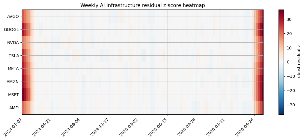
Visualization: AI infrastructure residual heatmap
The heatmap shows weekly residual z-scores by ticker after decomposition. Clusters suggest dates worth matching against launches, earnings, or macro events; edge-trimmed residual tables reduce first/last-window artifacts.
In [9]
residual_grid = components.copy()
residual_grid["residual_z"] = residual_grid.groupby("ticker")["residual"].transform(lambda s: (s - s.median()) / (1.4826 * (s - s.median()).abs().median() + 1e-12))
heat = residual_grid.pivot_table(index="ticker", columns="date", values="residual_z", aggfunc="mean").reindex(summary["ticker"].tolist()).dropna(how="all")
heat = heat.T
heat.index = pd.to_datetime(heat.index)
heat = heat.resample("W").mean().T
values = heat.to_numpy(dtype=float)
absmax = float(np.nanmax(np.abs(values))) if np.isfinite(values).any() else 1.0
fig, ax = plt.subplots(figsize=(11, 4.8))
im = ax.imshow(values, aspect="auto", cmap="RdBu_r", vmin=-absmax, vmax=absmax)
ax.set_yticks(range(len(heat.index)))
ax.set_yticklabels(heat.index)
tick_step = max(1, len(heat.columns) // 8)
xticks = list(range(0, len(heat.columns), tick_step))
ax.set_xticks(xticks)
ax.set_xticklabels([heat.columns[i].strftime("%Y-%m-%d") for i in xticks], rotation=45, ha="right")
ax.set_title("Weekly AI infrastructure residual z-score heatmap")
fig.colorbar(im, ax=ax, label="robust residual z")
plt.tight_layout()
plt.show()
image/png
6. Publication language
In [10]
phrasing = article_publication_phrasing()
phrasing
text/html
|
draft_claim |
evidence_based_phrasing |
| 0 |
This trend predicts the next price move. |
This trend summarizes the observed public seri... |
| 1 |
This model is better because it has more downl... |
Downloads are a public adoption proxy interpre... |
| 2 |
This repo is winning because stars are rising. |
Star velocity measures developer attention for... |
| 3 |
This pageview spike shows the topic matters most. |
Pageviews measure public attention during the ... |
| 4 |
This residual is a buy signal. |
This residual marks an event-like deviation fr... |
In [11]
save_table(source_card, "07_ai_infra_source_card")
save_table(basket_definition, "07_ai_infra_basket_definition")
save_table(audit, "07_ai_infra_market_audit")
save_table(summary, "07_ai_infra_component_summary")
save_table(returns, "07_ai_infra_return_proxy")
save_table(events, "07_ai_infra_residual_events")
save_table(phrasing, "07_ai_infra_publication_phrasing")
stdout
saved: examples/hot_trends/outputs/07_ai_infra_source_card.csv
saved: examples/hot_trends/outputs/07_ai_infra_basket_definition.csv
saved: examples/hot_trends/outputs/07_ai_infra_market_audit.csv
saved: examples/hot_trends/outputs/07_ai_infra_component_summary.csv
saved: examples/hot_trends/outputs/07_ai_infra_return_proxy.csv
saved: examples/hot_trends/outputs/07_ai_infra_residual_events.csv
saved: examples/hot_trends/outputs/07_ai_infra_publication_phrasing.csv