Seasonal-trend-dispersion decomposition
Seasonal-trend-dispersion decomposition
| Property | Value |
|---|---|
| Method | STD |
| Input mode | channelwise |
| Trend shape | (96,) |
| Notebook execution | ran |
| Reconstruction RMSE | 0.00000000 |
Notebook example metric: root mean square of input - (trend + season + residual) over all samples and channels. This checks additive bookkeeping; it is not a forecast error or a component-recovery score. The separate teaching input and intermediate arrays for the animation are linked below.
How it works
Method maturity: maintained. Implementation: native-backed.
STD represents each cycle using its mean, an L2 dispersion, and its own normalized shape.
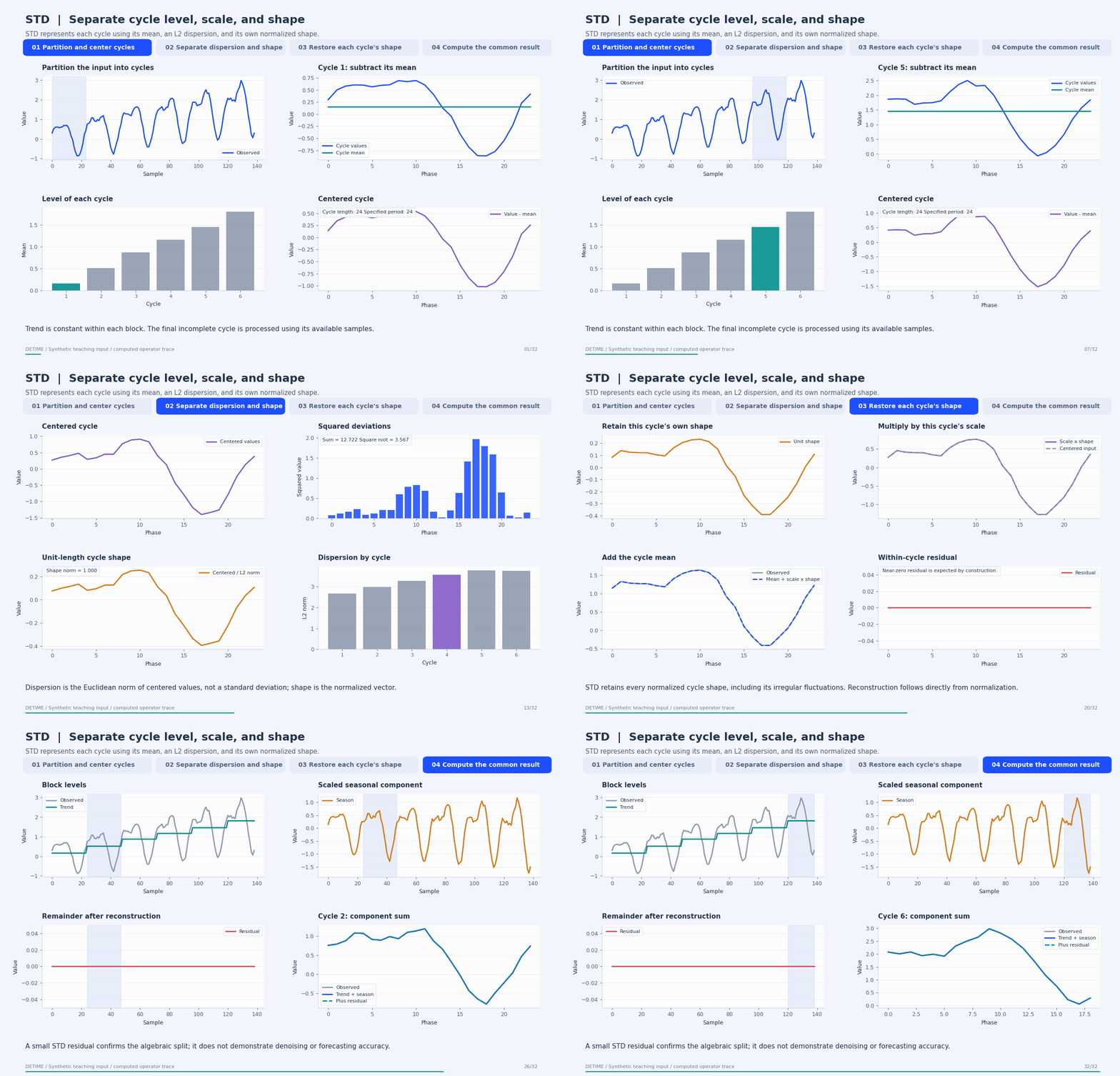
Deterministic synthetic teaching signal; not a benchmark.
Open GIF · Static PNG · Source arrays (NPZ) · Trace metadata
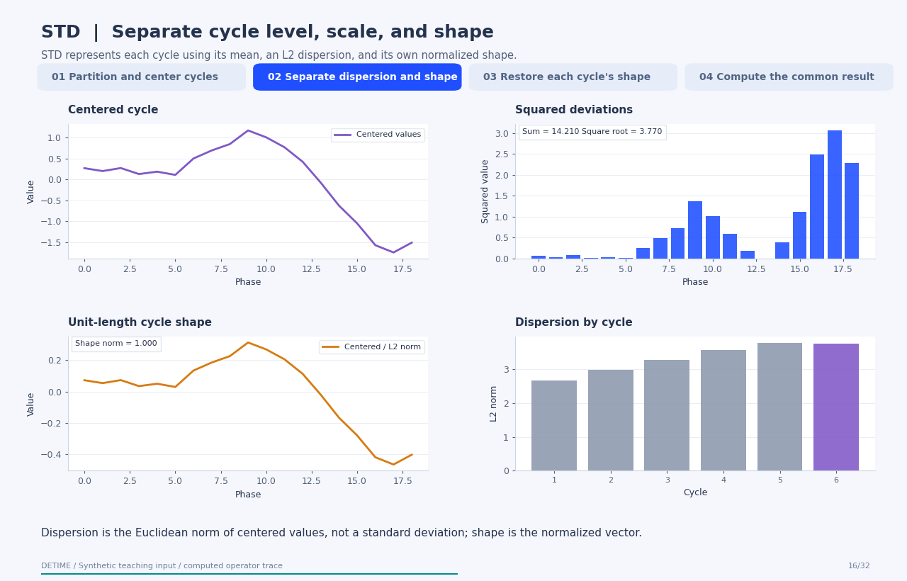
Follow the four steps
1. Partition and center cycles
Split at the configured period, compute each block's arithmetic mean, and subtract it. DeTime assigns that mean to every sample of the block, producing a piecewise-constant trend. A final partial block uses the samples that exist.
2. Separate dispersion and shape
Compute the Euclidean norm of each centered block as its dispersion. Divide by that norm to obtain a unit-length seasonal shape. A block whose norm is below eps receives zero dispersion and a zero shape.
3. Restore each cycle's shape
Multiply every cycle's own normalized shape by its own dispersion. This recovers the centered block, including irregular fluctuations. Add the block mean to reconstruct the observed values.
4. Compute the common result
Return trend, the scaled seasonal term, and residual = observed - trend - season, plus dispersion and seasonal-shape arrays. Residual is approximately zero by construction for nondegenerate blocks; this behavior is part of the representation and is not a denoising result.
Parameters that change the result
| Parameter | Effect on the computation |
|---|---|
period |
Block length and seasonal phase convention; a wrong period changes levels, scales, and shape alignment. |
eps |
Threshold below which a centered block is treated as having zero dispersion. |
max_period_search |
Upper bound on the FFT-based period heuristic used only when period is omitted; this animation supplies the period explicitly. |
What this animation computes
Every stage follows compute_std_components and the corresponding native kernel: block means, Euclidean norms, phase counts, and scaling. Both direct-source and public Python outputs are compared. The final short block is intentional.
Interpretation
- DeTime's STD/STDR use block means and L2 norms. Dispersion is not the sample standard deviation.
- STDR uses ordinary phase-wise means of normalized shapes. No robust loss, trimming, or outlier weights are used in this implementation.
- A partial cycle has its own mean and norm and contributes only available phases; its scale is not directly comparable to a full cycle without accounting for length.
- STD retains within-cycle irregular variation in its shape. STDR assigns deviations from a shared shape to the remainder.
- The supplied period and the starting phase define block boundaries; shifting the start changes the decomposition.
Try the method
Use this configuration with DecompositionConfig and decompose. The animation generator supplies the teaching input and records intermediate arrays.
{
  "method": "STD",
  "backend": "python",
  "params": {
    "period": 24
  }
}
See the configuration reference for the full interface and optional dependencies.
Sources and reproduction
- Dudek (2022), STD: A Seasonal-Trend-Dispersion Decomposition of Time Series
- DeTime implementation:
src/detime/methods/std.py - DeTime implementation:
native/src/std.cpp
Regenerate this animation with python scripts/generate_method_animations.py --methods STD.
The reproduction guide explains the environment,
numerical checks, coverage manifest, and how to inspect the stored arrays.
Code
case = CASES["STD"]
run_gallery_case("STD")
Output
STD: Fast seasonal-trend decomposition with dispersion-aware diagnostics.
status: ran
input mode: channelwise
trend shape: (96,)
backend: native
reconstruction RMSE: 0.00000000
Decomposition Plot
