Moving-average baseline
Moving-average baseline
| Property | Value |
|---|---|
| Method | MA_BASELINE |
| Input mode | univariate |
| Trend shape | (96,) |
| Notebook execution | ran |
| Reconstruction RMSE | 0.00000000 |
Notebook example metric: root mean square of input - (trend + season + residual) over all samples and channels. This checks additive bookkeeping; it is not a forecast error or a component-recovery score. The separate teaching input and intermediate arrays for the animation are linked below.
How it works
Method maturity: stable. Implementation: native-backed.
A centered uniform moving average supplies the trend; equal-phase means of the detrended series supply one repeated seasonal template.
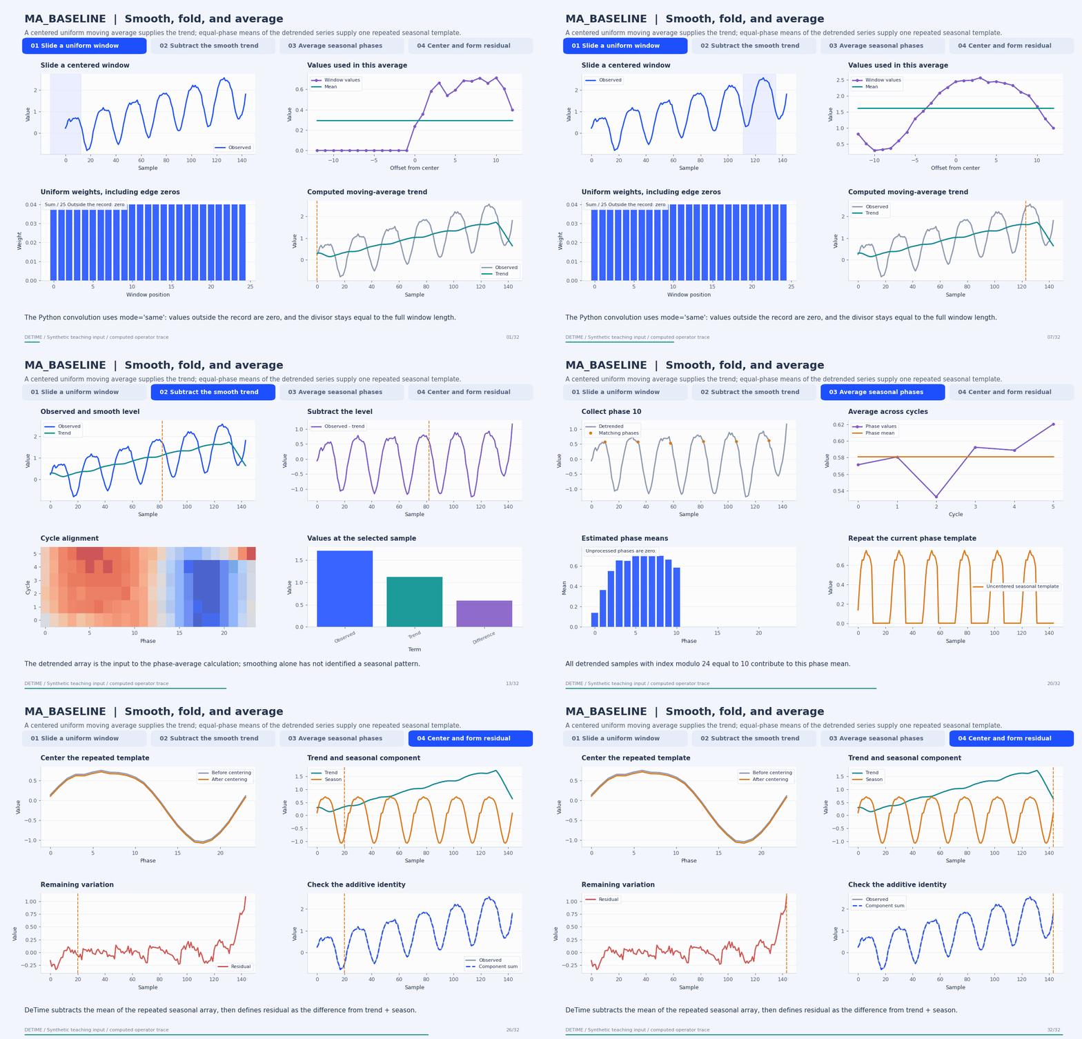
Deterministic synthetic teaching signal; not a benchmark.
Open GIF · Static PNG · Source arrays (NPZ) · Trace metadata
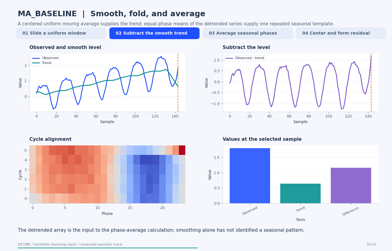
Follow the four steps
1. Slide a uniform window
Use uniform weights over an odd-length window. DeTime increments an even requested window by one. Its NumPy mode='same' convolution uses zero extension at both ends, so the divisor remains the full window length even near an edge.
2. Subtract the smooth trend
Compute detrended = observed - trend. Folding this array into cycle rows shows the values that share each seasonal phase.
3. Average seasonal phases
For each phase offset, average the detrended values separated by season_period samples. Repeat those means along the record. If season_period is omitted, the seasonal component is identically zero.
4. Center and form residual
Subtract the mean of the complete repeated seasonal array, then return residual = observed - trend - season. This guarantees an additive identity without establishing that each assigned component is physically correct.
Parameters that change the result
| Parameter | Effect on the computation |
|---|---|
trend_window |
Smoothing width; even requests are advanced to the next odd integer. The animation uses 25. |
season_period |
Spacing between observations assigned to the same seasonal phase; omitted means no seasonal estimate. |
What this animation computes
Window values, zero extension, uniform weights, phase averages, and centering follow the Python source. Final arrays are checked against the public Python execution path.
Interpretation
- This is an in-package baseline, not a reproduction of a separately published forecasting model.
- Zero extension pulls endpoint moving averages toward zero. Inspect boundary behavior before using the resulting components.
- One repeated phase template cannot express arbitrary cycle-to-cycle shape changes.
- Centered smoothing and full-record phase averaging use future observations relative to earlier time points; causal forecasting requires an origin-specific pipeline.
Try the method
Use this configuration with DecompositionConfig and decompose. The animation generator supplies the teaching input and records intermediate arrays.
{
  "method": "MA_BASELINE",
  "backend": "python",
  "params": {
    "trend_window": 25,
    "season_period": 24
  }
}
See the configuration reference for the full interface and optional dependencies.
Sources and reproduction
- DeTime moving-average baseline implementation
- DeTime implementation:
src/detime/methods/ma_baseline.py - DeTime implementation:
native/src/ma_baseline.cpp
Regenerate this animation with python scripts/generate_method_animations.py --methods MA_BASELINE.
The reproduction guide explains the environment,
numerical checks, coverage manifest, and how to inspect the stored arrays.
Code
case = CASES["MA_BASELINE"]
run_gallery_case("MA_BASELINE")
Output
MA_BASELINE: Simple moving-average baseline for smoke tests and lightweight workflows.
status: ran
input mode: univariate
trend shape: (96,)
backend: native
reconstruction RMSE: 0.00000000
Decomposition Plot
