Tutorial 05 - Pair spread decomposition and stat-arb
Executed tutorial notebook. This page is generated from
examples/notebooks/quant_trading/05_pairs_spread_decomposition_stat_arb.ipynb and includes markdown cells, code cells, stdout, tables, and captured figures from the committed notebook.
Tutorial Navigation
| Track | Tutorial notebook |
|---|---|
| Roadmap | Tutorial 00 - Roadmap |
| Strategy Lab | 01 Trend-Following Lab |
| Tutorial Sequence | 01 Real Market Data and Feature Factory |
| Tutorial Sequence | 02 Decomposition-aware MA and MACD |
| Strategy Lab | 02 Oscillation-Reversion Lab |
| Strategy Expansion | 03 Method-Specific Variants |
| Tutorial Sequence | 03 Residual Mean Reversion |
| Strategy Expansion | 04 Component Pair Trading |
| Tutorial Sequence | 04 Donchian Breakout |
| Tutorial Sequence | 05 Pair-Spread Stat-Arb |
| Tutorial Sequence | 06 Cross-Sectional Rotation |
| Native SSA Replay | 07 Native SSA High-Return / Low-Drawdown |
Executed Notebook
This notebook rewrites pairs trading around spread structure: rolling hedge ratio, spread trend drift, cycle timing and residual deviation.
In [1]
import matplotlib.pyplot as plt
import pandas as pd

from quant_trading.data import load_bundled_real_ohlcv_panel, ohlcv_audit_report
from quant_trading.strategy_pairs import (
    walkforward_pair_spread_features, pair_diagnostics, pair_feature_snapshot,
    make_classic_pair_weight_grid, make_detime_pair_weight_grid,
    compare_pair_suites, run_classical_pair_baselines, run_detime_pair_baselines,
)
from quant_trading.validation import turnover_report, compare_weight_strategies
1. Load real offline market data
In [2]
tickers = ["AUDUSD=X", "NZDUSD=X", "EURUSD=X", "GBPUSD=X"]
pairs = [("AUDUSD=X", "NZDUSD=X"), ("EURUSD=X", "GBPUSD=X")]
ohlcv = load_bundled_real_ohlcv_panel(tickers, min_observations=120)
ohlcv = {field: table.tail(760).copy() for field, table in ohlcv.items()}
prices = ohlcv["Close"]
ohlcv_audit_report(ohlcv)
text/html
| ticker | first_timestamp | last_timestamp | observations | close_missing_ratio | volume_missing_ratio | zero_volume_ratio | min_close | max_close | median_volume | |
|---|---|---|---|---|---|---|---|---|---|---|
| 0 | AUDUSD=X | 2015-02-02 | 2018-01-02 | 760 | 0.0 | 0.0 | 1.0 | 0.686106 | 0.811293 | 0.0 |
| 1 | NZDUSD=X | 2015-02-02 | 2018-01-02 | 760 | 0.0 | 0.0 | 1.0 | 0.626684 | 0.772380 | 0.0 |
| 2 | EURUSD=X | 2015-02-02 | 2018-01-02 | 760 | 0.0 | 0.0 | 1.0 | 1.039047 | 1.202906 | 0.0 |
| 3 | GBPUSD=X | 2015-02-02 | 2018-01-02 | 760 | 0.0 | 0.0 | 1.0 | 1.203935 | 1.588512 | 0.0 |
2. Build walk-forward spread decomposition features
In [3]
spread_features, spread_panel, beta_panel, pair_specs = walkforward_pair_spread_features(
    prices,
    pairs,
    hedge_window=126,
    method="STL",
    period=126,
    train_window=504,
    step=5,
    z_window=63,
)
spread_panel.tail()
text/html
| AUDUSD=X__NZDUSD=X | EURUSD=X__GBPUSD=X | |
|---|---|---|
| Date | ||
| 2017-12-27 | -0.078105 | 0.055287 |
| 2017-12-28 | -0.073091 | 0.057506 |
| 2017-12-29 | -0.072003 | 0.060825 |
| 2018-01-01 | -0.072259 | 0.062524 |
| 2018-01-02 | -0.071041 | 0.063328 |
In [4]
pair_diagnostics(prices, pair_specs, hedge_window=90)
text/html
| pair | date | spread | beta | pair_corr_120 | spread_trend_slope | spread_cycle_slope | spread_residual_z | spread_residual_abs_z | volume_liquidity_ok | |
|---|---|---|---|---|---|---|---|---|---|---|
| 0 | AUDUSD=X/NZDUSD=X | 2018-01-02 | -0.092184 | 0.453700 | 0.632244 | -0.000494 | 0.002530 | -0.386195 | 0.386195 | True |
| 1 | EURUSD=X/GBPUSD=X | 2018-01-02 | 0.076336 | 0.355382 | 0.446730 | 0.000147 | 0.002752 | 1.196764 | 1.196764 | True |
In [5]
snapshot = pair_feature_snapshot(spread_features, tail=2)
snapshot.query("feature in ['trend_slope', 'cycle_slope', 'residual_z', 'residual_abs_z']").tail(16)
text/html
| date | pair | feature | value | |
|---|---|---|---|---|
| 8 | 2018-01-01 | AUDUSD=X__NZDUSD=X | cycle_slope | -0.000361 |
| 9 | 2018-01-01 | EURUSD=X__GBPUSD=X | cycle_slope | 0.000803 |
| 10 | 2018-01-02 | AUDUSD=X__NZDUSD=X | cycle_slope | -0.000361 |
| 11 | 2018-01-02 | EURUSD=X__GBPUSD=X | cycle_slope | 0.000803 |
| 12 | 2018-01-01 | AUDUSD=X__NZDUSD=X | residual_abs_z | 2.174176 |
| 13 | 2018-01-01 | EURUSD=X__GBPUSD=X | residual_abs_z | 0.840480 |
| 14 | 2018-01-02 | AUDUSD=X__NZDUSD=X | residual_abs_z | 2.174176 |
| 15 | 2018-01-02 | EURUSD=X__GBPUSD=X | residual_abs_z | 0.840480 |
| 16 | 2018-01-01 | AUDUSD=X__NZDUSD=X | residual_z | 2.174176 |
| 17 | 2018-01-01 | EURUSD=X__GBPUSD=X | residual_z | -0.840480 |
| 18 | 2018-01-02 | AUDUSD=X__NZDUSD=X | residual_z | 2.174176 |
| 19 | 2018-01-02 | EURUSD=X__GBPUSD=X | residual_z | -0.840480 |
| 64 | 2018-01-01 | AUDUSD=X__NZDUSD=X | trend_slope | -0.000070 |
| 65 | 2018-01-01 | EURUSD=X__GBPUSD=X | trend_slope | 0.000351 |
| 66 | 2018-01-02 | AUDUSD=X__NZDUSD=X | trend_slope | -0.000070 |
| 67 | 2018-01-02 | EURUSD=X__GBPUSD=X | trend_slope | 0.000351 |
3. Backtest classical baselines and DeTime rewrites
In [6]
classic_weights = make_classic_pair_weight_grid(prices, pairs=pairs, lookback=90)
detime_weights = make_detime_pair_weight_grid(prices, pair_specs, spread_features, spread_panel=spread_panel, beta_panel=beta_panel)
all_weights = {**classic_weights, **detime_weights}
comparison, results = compare_weight_strategies(prices, all_weights, fee_bps=1.0, slippage_bps=2.0)
comparison.insert(0, "strategy_group", ["detime_pair" if str(idx).startswith("detime") else "classical_pair" for idx in comparison.index])
comparison[["strategy_group", "cagr", "sharpe", "max_drawdown", "average_turnover"]].round(4)
text/html
| strategy_group | cagr | sharpe | max_drawdown | average_turnover | |
|---|---|---|---|---|---|
| strategy | |||||
| classic_pair_ratio_zscore_120 | classical_pair | 0.0162 | 0.4520 | -0.0338 | 0.0671 |
| classic_pair_corr_filtered_zscore | classical_pair | -0.0114 | -0.3120 | -0.0687 | 0.0499 |
| classic_pair_spread_zscore_120 | classical_pair | -0.0140 | -0.3748 | -0.0687 | 0.0540 |
| detime_spread_cycle_timed | detime_pair | -0.0158 | -0.7761 | -0.0511 | 0.0146 |
| detime_spread_trend_drift_blocker | detime_pair | -0.0155 | -0.8349 | -0.0575 | 0.0186 |
| detime_spread_residual_z | detime_pair | -0.0176 | -0.9479 | -0.0575 | 0.0186 |
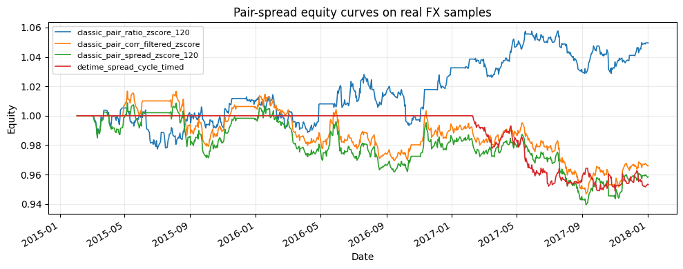
In [7]
leaders = comparison.sort_values("sharpe", ascending=False).head(4).index
fig, ax = plt.subplots(figsize=(10, 4))
for name in leaders:
    results[name].equity.plot(ax=ax, linewidth=1.2, label=name)
ax.set_title("Pair-spread equity curves on real FX samples")
ax.set_ylabel("Equity")
ax.legend(loc="best", fontsize=8)
ax.grid(True, alpha=0.25)
plt.tight_layout()
plt.show()
image/png
In [8]
turnover_report(all_weights).round(4)
text/html
| average_turnover | median_turnover | max_turnover | average_gross_exposure | |
|---|---|---|---|---|
| strategy | ||||
| classic_pair_spread_zscore_120 | 0.0540 | 0.0037 | 2.0 | 0.8632 |
| classic_pair_corr_filtered_zscore | 0.0499 | 0.0035 | 2.0 | 0.8171 |
| classic_pair_ratio_zscore_120 | 0.0671 | 0.0000 | 1.0 | 0.8303 |
| detime_spread_residual_z | 0.0186 | 0.0000 | 2.0 | 0.3118 |
| detime_spread_cycle_timed | 0.0146 | 0.0000 | 2.0 | 0.2987 |
| detime_spread_trend_drift_blocker | 0.0186 | 0.0000 | 2.0 | 0.3250 |
4. Live-data extension
Run run_column_05_pairs_spread_decomposition.py without --use-bundled-sample and pass pairs such as KO:PEP, XOM:CVX, MA:V, or SPY:QQQ.