Wikimedia Attention and Hype Decay
Executed tutorial notebook. This page is generated from
examples/notebooks/hot_trends/05_wikipedia_attention_hype_decay.ipynb and includes markdown cells, code cells, stdout, tables, and captured figures from the committed notebook.
Executed Notebook
This notebook uses Wikimedia Analytics API pageviews to measure public attention cycles. Pageviews are interpreted as public-attention signals.
Data sources are recorded in the source audit table.
In [1]
from pathlib import Path
import os

import matplotlib.pyplot as plt
import numpy as np
import pandas as pd

from examples.hot_trends.data import (
    HotTrendDataError,
    append_real_snapshot,
    build_arxiv_monthly_counts,
    fetch_coingecko_market_chart,
    fetch_defillama_stablecoin_chains,
    fetch_github_repo_metadata,
    fetch_github_stargazers,
    fetch_huggingface_models,
    fetch_wikipedia_pageviews,
    source_audit_table,
)
from examples.hot_trends.decomposition import (
    component_summary,
    decompose_table,
    editorial_priority,
    residual_event_table,
)
from examples.hot_trends.scoring import article_publication_phrasing

pd.set_option("display.max_columns", 80)
pd.set_option("display.max_rows", 80)
plt.rcParams.update({"axes.grid": True})

CACHE_DIR = Path("examples/hot_trends/cache")
OUTPUT_DIR = Path("examples/hot_trends/outputs")
CACHE_DIR.mkdir(parents=True, exist_ok=True)
OUTPUT_DIR.mkdir(parents=True, exist_ok=True)

def save_table(df, name):
    path = OUTPUT_DIR / f"{name}.csv"
    df.to_csv(path, index=False)
    print(f"saved: {path.as_posix()}")
1. Select pages and date window
In [2]
articles = [
    "Artificial intelligence",
    "Large language model",
    "ChatGPT",
    "Bitcoin",
    "Nvidia",
    "OpenAI",
]
START = "2025-01-01"
END = "2026-05-20"
pd.DataFrame({"article": articles})
text/html
| article | |
|---|---|
| 0 | Artificial intelligence |
| 1 | Large language model |
| 2 | ChatGPT |
| 3 | Bitcoin |
| 4 | Nvidia |
| 5 | OpenAI |
2. Fetch pageviews
In [3]
frames = []
for article in articles:
    frames.append(fetch_wikipedia_pageviews(article, start=START, end=END))
views = pd.concat(frames, ignore_index=True)
views.head(20)
text/html
| date | article | views | project | source | data_quality | |
|---|---|---|---|---|---|---|
| 0 | 2025-01-01 | Artificial intelligence | 9447 | en.wikipedia.org | Wikimedia Analytics API | public_api_snapshot |
| 1 | 2025-01-02 | Artificial intelligence | 10777 | en.wikipedia.org | Wikimedia Analytics API | public_api_snapshot |
| 2 | 2025-01-03 | Artificial intelligence | 10148 | en.wikipedia.org | Wikimedia Analytics API | public_api_snapshot |
| 3 | 2025-01-04 | Artificial intelligence | 9172 | en.wikipedia.org | Wikimedia Analytics API | public_api_snapshot |
| 4 | 2025-01-05 | Artificial intelligence | 8865 | en.wikipedia.org | Wikimedia Analytics API | public_api_snapshot |
| 5 | 2025-01-06 | Artificial intelligence | 11022 | en.wikipedia.org | Wikimedia Analytics API | public_api_snapshot |
| 6 | 2025-01-07 | Artificial intelligence | 12419 | en.wikipedia.org | Wikimedia Analytics API | public_api_snapshot |
| 7 | 2025-01-08 | Artificial intelligence | 12421 | en.wikipedia.org | Wikimedia Analytics API | public_api_snapshot |
| 8 | 2025-01-09 | Artificial intelligence | 12147 | en.wikipedia.org | Wikimedia Analytics API | public_api_snapshot |
| 9 | 2025-01-10 | Artificial intelligence | 11222 | en.wikipedia.org | Wikimedia Analytics API | public_api_snapshot |
| 10 | 2025-01-11 | Artificial intelligence | 8817 | en.wikipedia.org | Wikimedia Analytics API | public_api_snapshot |
| 11 | 2025-01-12 | Artificial intelligence | 9058 | en.wikipedia.org | Wikimedia Analytics API | public_api_snapshot |
| 12 | 2025-01-13 | Artificial intelligence | 13942 | en.wikipedia.org | Wikimedia Analytics API | public_api_snapshot |
| 13 | 2025-01-14 | Artificial intelligence | 12763 | en.wikipedia.org | Wikimedia Analytics API | public_api_snapshot |
| 14 | 2025-01-15 | Artificial intelligence | 13336 | en.wikipedia.org | Wikimedia Analytics API | public_api_snapshot |
| 15 | 2025-01-16 | Artificial intelligence | 13364 | en.wikipedia.org | Wikimedia Analytics API | public_api_snapshot |
| 16 | 2025-01-17 | Artificial intelligence | 11866 | en.wikipedia.org | Wikimedia Analytics API | public_api_snapshot |
| 17 | 2025-01-18 | Artificial intelligence | 9003 | en.wikipedia.org | Wikimedia Analytics API | public_api_snapshot |
| 18 | 2025-01-19 | Artificial intelligence | 9598 | en.wikipedia.org | Wikimedia Analytics API | public_api_snapshot |
| 19 | 2025-01-20 | Artificial intelligence | 11688 | en.wikipedia.org | Wikimedia Analytics API | public_api_snapshot |
3. Audit the pageview table
In [4]
audit = source_audit_table(views, value_col="views", entity_col="article", time_col="date")
audit
text/html
| series | first_timestamp | last_timestamp | observations | missing_ratio | min_value | max_value | |
|---|---|---|---|---|---|---|---|
| 0 | Artificial intelligence | 2025-01-01 00:00:00 | 2026-05-20 00:00:00 | 505 | 0.0 | 6726.0 | 47069.0 |
| 1 | Bitcoin | 2025-01-01 00:00:00 | 2026-05-20 00:00:00 | 505 | 0.0 | 2241.0 | 18494.0 |
| 2 | ChatGPT | 2025-01-01 00:00:00 | 2026-05-20 00:00:00 | 505 | 0.0 | 33844.0 | 832465.0 |
| 3 | Large language model | 2025-01-01 00:00:00 | 2026-05-20 00:00:00 | 505 | 0.0 | 1965.0 | 11498.0 |
| 4 | Nvidia | 2025-01-01 00:00:00 | 2026-05-20 00:00:00 | 505 | 0.0 | 3163.0 | 68291.0 |
| 5 | OpenAI | 2025-01-01 00:00:00 | 2026-05-20 00:00:00 | 505 | 0.0 | 4652.0 | 53724.0 |
4. Decompose pageview attention
In [5]
components = decompose_table(views, entity_col="article", time_col="date", value_col="views", method="MA_BASELINE", period=7, trend_window=21, transform="log1p")
summary = editorial_priority(component_summary(components, entity_col="article", time_col="date"), entity_col="article")
summary
text/html
| article | observations | first_timestamp | last_timestamp | trend_last | trend_slope_per_step | cycle_strength_proxy | residual_std | max_abs_residual_z | method | trend_slope_per_step_rank_pct | cycle_strength_proxy_rank_pct | max_abs_residual_z_rank_pct | editorial_priority_score | |
|---|---|---|---|---|---|---|---|---|---|---|---|---|---|---|
| 0 | Artificial intelligence | 505 | 2025-01-01 00:00:00 | 2026-05-20 00:00:00 | 4.882320 | -0.000011 | -6.502693 | 0.544259 | 55.176621 | MA_BASELINE | 1.000000 | 0.166667 | 0.833333 | 0.758333 |
| 3 | Large language model | 505 | 2025-01-01 00:00:00 | 2026-05-20 00:00:00 | 4.231900 | -0.000431 | -3.389617 | 0.470944 | 59.617727 | MA_BASELINE | 0.500000 | 0.333333 | 1.000000 | 0.691667 |
| 2 | ChatGPT | 505 | 2025-01-01 00:00:00 | 2026-05-20 00:00:00 | 5.828161 | -0.000429 | -1.903450 | 0.698960 | 46.942855 | MA_BASELINE | 0.666667 | 0.666667 | 0.666667 | 0.666667 |
| 4 | Nvidia | 505 | 2025-01-01 00:00:00 | 2026-05-20 00:00:00 | 4.882153 | -0.000056 | -1.019794 | 0.605797 | 23.278477 | MA_BASELINE | 0.833333 | 1.000000 | 0.166667 | 0.566667 |
| 5 | OpenAI | 505 | 2025-01-01 00:00:00 | 2026-05-20 00:00:00 | 4.726995 | -0.000514 | -2.325489 | 0.555429 | 40.235922 | MA_BASELINE | 0.333333 | 0.500000 | 0.500000 | 0.441667 |
| 1 | Bitcoin | 505 | 2025-01-01 00:00:00 | 2026-05-20 00:00:00 | 4.202332 | -0.001413 | -1.550364 | 0.527478 | 33.181356 | MA_BASELINE | 0.166667 | 0.833333 | 0.333333 | 0.375000 |
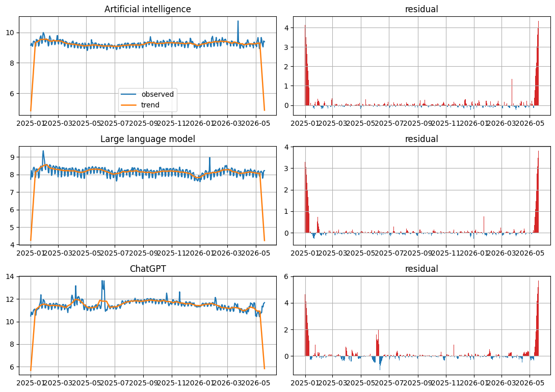
Visualization: Wikimedia attention components
Top article panels reveal the transformed pageview trend and residual attention shocks.
In [6]
top_articles = summary["article"].head(3).tolist()
fig, axes = plt.subplots(len(top_articles), 2, figsize=(11, max(3.0, 2.6 * len(top_articles))), squeeze=False)
for row, article in enumerate(top_articles):
    panel = components.loc[components["article"].eq(article)].sort_values("date").copy()
    panel["date"] = pd.to_datetime(panel["date"])
    axes[row, 0].plot(panel["date"], panel["observed"], label="observed", linewidth=1.6)
    axes[row, 0].plot(panel["date"], panel["trend"], label="trend", linewidth=1.8)
    axes[row, 0].set_title(article)
    axes[row, 1].bar(panel["date"], panel["residual"], color=np.where(panel["residual"] >= 0, "tab:red", "tab:blue"), width=1.0)
    axes[row, 1].set_title("residual")
axes[0, 0].legend(loc="best")
plt.tight_layout()
plt.show()
image/png
5. Residual shock events
In [7]
events = residual_event_table(components, entity_col="article", time_col="date", top_n=25)
events
text/html
| date | article | observed | trend | season | residual | residual_z | abs_residual_z | method | |
|---|---|---|---|---|---|---|---|---|---|
| 0 | 2026-05-20 | Large language model | 8.218787 | 4.231900 | 0.178067 | 3.808820 | 59.617727 | 59.617727 | MA_BASELINE |
| 1 | 2026-05-20 | Artificial intelligence | 9.388487 | 4.882320 | 0.159566 | 4.346601 | 55.176621 | 55.176621 | MA_BASELINE |
| 2 | 2026-05-19 | Large language model | 8.216358 | 4.609306 | 0.126721 | 3.480331 | 54.475977 | 54.475977 | MA_BASELINE |
| 3 | 2025-01-02 | Large language model | 8.220403 | 4.627593 | 0.113499 | 3.479311 | 54.460007 | 54.460007 | MA_BASELINE |
| 4 | 2025-01-01 | Artificial intelligence | 9.153558 | 4.850246 | 0.159566 | 4.143747 | 52.605795 | 52.605795 | MA_BASELINE |
| 5 | 2025-01-01 | Large language model | 7.724888 | 4.248696 | 0.178067 | 3.298125 | 51.623946 | 51.623946 | MA_BASELINE |
| 6 | 2026-05-19 | Artificial intelligence | 9.428190 | 5.308164 | 0.116739 | 4.003287 | 50.825719 | 50.825719 | MA_BASELINE |
| 7 | 2025-01-02 | Artificial intelligence | 9.285262 | 5.284128 | 0.078876 | 3.922259 | 49.798823 | 49.798823 | MA_BASELINE |
| 8 | 2026-05-18 | Large language model | 8.167919 | 4.994446 | 0.086805 | 3.086668 | 48.314061 | 48.314061 | MA_BASELINE |
| 9 | 2025-01-03 | Large language model | 8.076826 | 5.023572 | 0.007082 | 3.046172 | 47.680178 | 47.680178 | MA_BASELINE |
| 10 | 2026-05-20 | ChatGPT | 11.680802 | 5.828161 | 0.179541 | 5.673099 | 46.942855 | 46.942855 | MA_BASELINE |
| 11 | 2026-05-18 | Artificial intelligence | 9.439784 | 5.750124 | 0.058516 | 3.631144 | 46.109457 | 46.109457 | MA_BASELINE |
| 12 | 2025-01-03 | Artificial intelligence | 9.225130 | 5.738544 | -0.016744 | 3.503331 | 44.489646 | 44.489646 | MA_BASELINE |
| 13 | 2026-05-17 | Large language model | 7.886833 | 5.385132 | -0.243808 | 2.745509 | 42.973970 | 42.973970 | MA_BASELINE |
| 14 | 2026-05-19 | ChatGPT | 11.619068 | 6.325335 | 0.130722 | 5.163010 | 42.724622 | 42.724622 | MA_BASELINE |
| 15 | 2025-01-04 | Large language model | 7.850493 | 5.417504 | -0.270839 | 2.703828 | 42.321549 | 42.321549 | MA_BASELINE |
| 16 | 2026-05-20 | OpenAI | 9.355825 | 4.726995 | 0.181937 | 4.446893 | 40.235922 | 40.235922 | MA_BASELINE |
| 17 | 2025-01-04 | Artificial intelligence | 9.124020 | 6.188752 | -0.205570 | 3.140837 | 39.895677 | 39.895677 | MA_BASELINE |
| 18 | 2026-05-18 | ChatGPT | 11.599002 | 6.833267 | 0.068988 | 4.696747 | 38.868815 | 38.868815 | MA_BASELINE |
| 19 | 2026-05-17 | Artificial intelligence | 9.048645 | 6.199097 | -0.193600 | 3.043147 | 38.657630 | 38.657630 | MA_BASELINE |
| 20 | 2025-01-01 | ChatGPT | 10.491830 | 5.674245 | 0.179541 | 4.638044 | 38.383364 | 38.383364 | MA_BASELINE |
| 21 | 2025-01-02 | ChatGPT | 10.846693 | 6.177299 | 0.067253 | 4.602141 | 38.086459 | 38.086459 | MA_BASELINE |
| 22 | 2026-05-19 | OpenAI | 9.408371 | 5.141967 | 0.124530 | 4.141875 | 37.489449 | 37.489449 | MA_BASELINE |
| 23 | 2025-01-01 | OpenAI | 8.955319 | 4.735431 | 0.181937 | 4.037952 | 36.553695 | 36.553695 | MA_BASELINE |
| 24 | 2025-01-05 | Large language model | 7.901007 | 5.813074 | -0.243808 | 2.331741 | 36.497361 | 36.497361 | MA_BASELINE |
6. Hype-decay table
A simple decay proxy: after each article's largest residual event, count days until residual drops below half of that peak.
In [8]
decay_rows = []
for article, sub in components.groupby("article"):
    sub = sub.sort_values("date").copy()
    rz = (sub["residual"] - sub["residual"].median()).abs()
    peak_idx = int(rz.idxmax())
    peak_date = pd.to_datetime(sub.loc[peak_idx, "date"])
    peak = float(rz.loc[peak_idx])
    after = sub.loc[peak_idx:].copy()
    after_rz = (after["residual"] - sub["residual"].median()).abs()
    below = after.loc[after_rz <= 0.5 * peak]
    half_life_days = None if below.empty else int((pd.to_datetime(below["date"].iloc[0]) - peak_date).days)
    decay_rows.append({"article": article, "peak_date": str(peak_date.date()), "peak_residual_abs": peak, "attention_half_life_days": half_life_days})
decay = pd.DataFrame(decay_rows).sort_values("peak_residual_abs", ascending=False)
decay
text/html
| article | peak_date | peak_residual_abs | attention_half_life_days | |
|---|---|---|---|---|
| 2 | ChatGPT | 2026-05-20 | 5.676558 | NaN |
| 5 | OpenAI | 2026-05-20 | 4.468527 | NaN |
| 0 | Artificial intelligence | 2026-05-20 | 4.353788 | NaN |
| 4 | Nvidia | 2026-05-20 | 4.332644 | NaN |
| 1 | Bitcoin | 2025-01-01 | 4.162031 | 6.0 |
| 3 | Large language model | 2026-05-20 | 3.808767 | NaN |
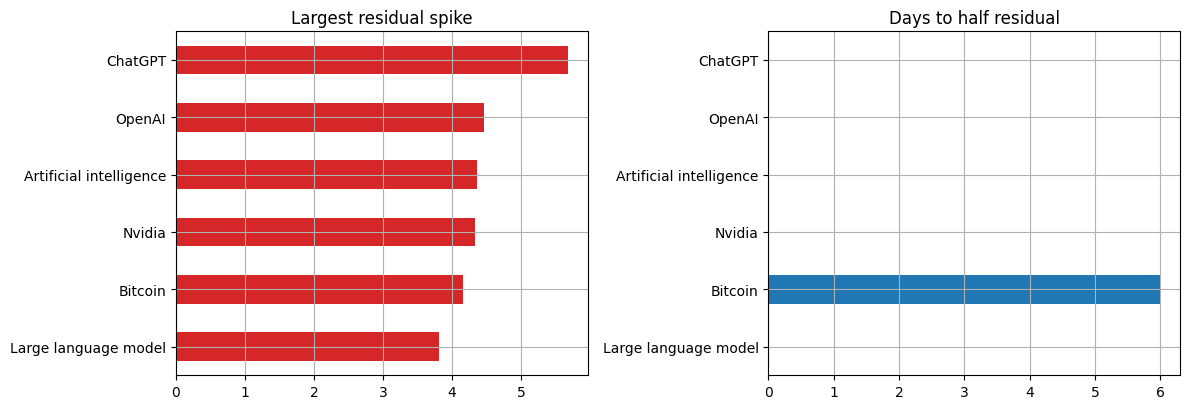
Visualization: hype decay half-life
The bar chart exposes which attention spikes decayed quickly and which stayed elevated or remain unresolved.
In [9]
decay_plot = decay.copy()
decay_plot["attention_half_life_days"] = pd.to_numeric(decay_plot["attention_half_life_days"], errors="coerce")
decay_plot = decay_plot.sort_values("peak_residual_abs")
fig, axes = plt.subplots(1, 2, figsize=(12, 4.2))
decay_plot.plot(kind="barh", x="article", y="peak_residual_abs", ax=axes[0], color="tab:red", legend=False, title="Largest residual spike")
decay_plot.assign(attention_half_life_days=decay_plot["attention_half_life_days"].fillna(0)).plot(kind="barh", x="article", y="attention_half_life_days", ax=axes[1], color="tab:blue", legend=False, title="Days to half residual")
axes[0].set_ylabel("")
axes[1].set_ylabel("")
plt.tight_layout()
plt.show()
image/png
In [10]
save_table(audit, "05_wikipedia_attention_audit")
save_table(summary, "05_wikipedia_attention_summary")
save_table(events, "05_wikipedia_attention_events")
save_table(decay, "05_wikipedia_hype_decay")
save_table(article_publication_phrasing(), "05_wikipedia_publication_phrasing")
stdout
saved: examples/hot_trends/outputs/05_wikipedia_attention_audit.csv
saved: examples/hot_trends/outputs/05_wikipedia_attention_summary.csv
saved: examples/hot_trends/outputs/05_wikipedia_attention_events.csv
saved: examples/hot_trends/outputs/05_wikipedia_hype_decay.csv
saved: examples/hot_trends/outputs/05_wikipedia_publication_phrasing.csv