Variational mode decomposition
Variational mode decomposition
| Property | Value |
|---|---|
| Method | VMD |
| Input mode | univariate |
| Trend shape | (96,) |
| Notebook execution | ran |
| Reconstruction RMSE | 0.00000000 |
Notebook example metric: root mean square of input - (trend + season + residual) over all samples and channels. This checks additive bookkeeping; it is not a forecast error or a component-recovery score. The separate teaching input and intermediate arrays for the animation are linked below.
How it works
Method maturity: stable. Implementation: native-backed.
VMD alternates between frequency-domain mode updates and spectral-energy centers. DeTime's grouping into trend and season is a separate step after this optimization.
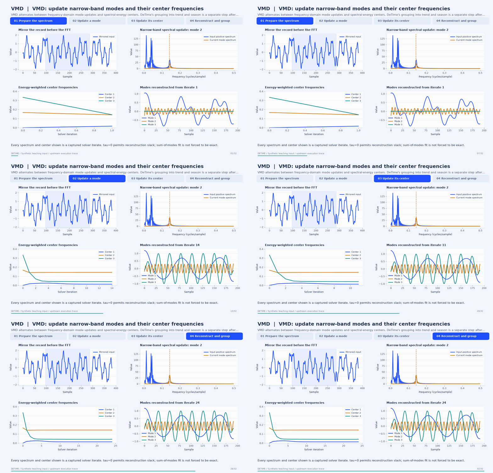
Deterministic synthetic teaching signal; not a benchmark.
Open GIF · Static PNG · Source arrays (NPZ) · Trace metadata
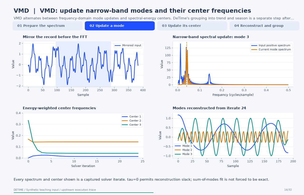
Follow the four steps
1. Prepare the spectrum
Mirror the signal, compute its FFT, and retain the positive-frequency representation.
2. Update a mode
Fit the remaining spectrum with a bandwidth penalty around the current center frequency.
3. Update its center
Use the mode's positive-frequency energy to update its center, then repeat across modes.
4. Reconstruct and group
Complete the conjugate spectrum, invert the FFT, crop the mirrored margins, and group modes.
Parameters that change the result
| Parameter | Effect on the computation |
|---|---|
K |
Number of modes; the demonstration uses 3. |
alpha |
Penalizes spectral spread around each center; the demonstration uses 1500. |
tau |
Dual-update step; zero permits noise slack and does not enforce an exact sum of modes. |
init / tol |
Initialization and convergence tolerance affect the computed solution. |
What this animation computes
Captured vmdpy 0.2 loop arrays without changing solver updates; intermediate time-domain modes use its conjugate-completion and mirror-cropping convention.
Interpretation
- The animation captures the optional vmdpy path; the native path has its own implementation and iteration control.
- Center frequencies shown here are raw solver frequencies in cycles/sample, not DeTime's converted metadata field.
- VMD modes need a grouping rule before being named trend or season; frequency ordering is not a physical-source guarantee.
Try the method
Use this configuration with DecompositionConfig and decompose. The animation generator supplies the teaching input and records intermediate arrays.
{
  "method": "VMD",
  "params": {
    "K": 3,
    "alpha": 1500.0,
    "tau": 0.0,
    "init": 1,
    "tol": 1e-07,
    "primary_period": 24
  },
  "backend": "python"
}
See the configuration reference for the full interface and optional dependencies.
Sources and reproduction
- Original VMD paper
- vmdpy reference implementation
- Maintained sktime continuation
- DeTime implementation:
src/detime/methods/vmd.py - DeTime implementation:
native/src/vmd.cpp
Regenerate this animation with python scripts/generate_method_animations.py --methods VMD.
The reproduction guide explains the environment,
numerical checks, coverage manifest, and how to inspect the stored arrays.
Code
case = CASES["VMD"]
run_gallery_case("VMD")
Output
VMD: Variational mode decomposition integrated into the common workflow layer.
status: ran
input mode: univariate
trend shape: (96,)
backend: native
reconstruction RMSE: 0.00000000
Decomposition Plot
