Experimental Gabor clustering path
Experimental Gabor clustering path
| Property | Value |
|---|---|
| Method | GABOR_CLUSTER |
| Input mode | univariate |
| Trend shape | `` |
| Notebook execution | skipped |
| Reconstruction RMSE | n/a |
Notebook example metric: root mean square of input - (trend + season + residual) over all samples and channels. This checks additive bookkeeping; it is not a forecast error or a component-recovery score. The separate teaching input and intermediate arrays for the animation are linked below.
How it works
Method maturity: experimental. Implementation: native-backed.
DeTime's experimental operator builds windowed Fourier atoms, assigns their features to a supplied codebook, and reconstructs cluster-specific contributions with overlap-add.
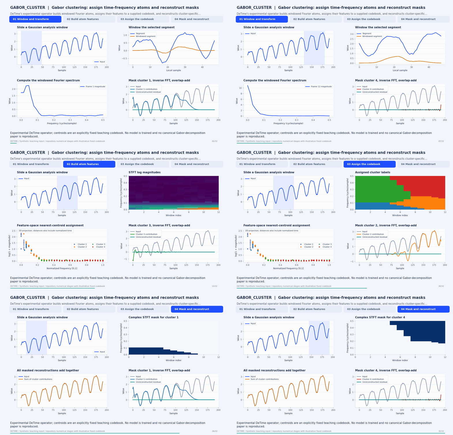
Deterministic synthetic teaching signal; not a benchmark.
Open GIF · Static PNG · Source arrays (NPZ) · Trace metadata
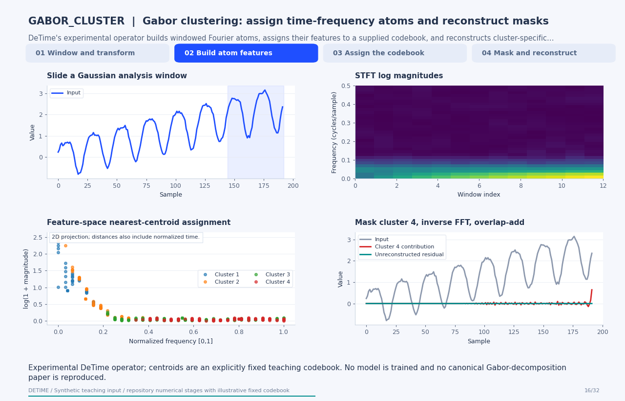
Follow the four steps
1. Window and transform
Slide the normalized Gaussian window and compute real FFT coefficients.
2. Build atom features
Represent each time-frequency bin by normalized time, normalized frequency, and log amplitude.
3. Assign the codebook
Standardize features with the stored mean/scale and select the nearest supplied centroid.
4. Mask and reconstruct
Retain each cluster's complex coefficients, apply inverse FFT and normalized overlap-add, then group contributions heuristically.
Parameters that change the result
| Parameter | Effect on the computation |
|---|---|
model / model_path |
A supplied GaborClusterModel is required; the decomposition function does not train a codebook. |
win_len / hop / n_fft |
Stored in the model; the example uses 48/12/64 and a Gaussian window. |
max_clusters |
Optionally retains the highest-energy clusters before reconstruction. |
trend_freq_thr |
Heuristic threshold on the de-standardized centroid frequency, normalized from zero to Nyquist. |
What this animation computes
Uses the current repository's window, STFT, feature extraction and inverse-overlap-add functions. Squared Euclidean assignment matches the supplied-centroid operation; native cluster reconstructions are independently compared when available. Model normalization, fixed teaching centroids, and numeric window settings are saved with the trace. The public call requires a GaborClusterModel or a model archive created with its save() method; the generic config is incomplete until that model is supplied.
Interpretation
- This is an experimental, repository-specific operator, not a claimed reproduction of a canonical forecasting or decomposition architecture.
- The fixed four-centroid teaching codebook is neither trained nor evidence of a useful scientific clustering.
- The current frame grid can leave an uncovered tail when the record length is not aligned with the hop; the residual retains that difference.
- Cluster labels are codebook labels; assigning low-frequency clusters to trend is a heuristic.
Try the method
The public method requires a GaborClusterModel object or a saved model_path. The animation generator constructs an explicitly fixed teaching codebook; the arrays are included in its source archive. Supply a model before calling decompose with the configuration below.
{
  "method": "GABOR_CLUSTER",
  "params": {
    "trend_freq_thr": 0.08
  }
}
See the configuration reference for the full interface and optional dependencies.
Sources and reproduction
- DeTime Gabor operator source
- DeTime native Gabor kernels
- DeTime implementation:
src/detime/methods/gabor_cluster.py - DeTime implementation:
native/src/gabor.cpp
Regenerate this animation with python scripts/generate_method_animations.py --methods GABOR_CLUSTER.
The reproduction guide explains the environment,
numerical checks, coverage manifest, and how to inspect the stored arrays.
Code
case = CASES["GABOR_CLUSTER"]
print(case["skip"])
Output
requires a trained GaborClusterModel or model_path plus the experimental clustering backend