Tutorial 04 - Donchian and Turtle breakout with DeTime volume confirmation
examples/notebooks/quant_trading/04_turtle_donchian_breakout_volume_confirmation.ipynb and includes markdown cells, code cells, stdout, tables, and captured figures from the committed notebook.
Tutorial Navigation
| Track | Tutorial notebook |
|---|---|
| Roadmap | Tutorial 00 - Roadmap |
| Strategy Lab | 01 Trend-Following Lab |
| Tutorial Sequence | 01 Real Market Data and Feature Factory |
| Tutorial Sequence | 02 Decomposition-aware MA and MACD |
| Strategy Lab | 02 Oscillation-Reversion Lab |
| Strategy Expansion | 03 Method-Specific Variants |
| Tutorial Sequence | 03 Residual Mean Reversion |
| Strategy Expansion | 04 Component Pair Trading |
| Tutorial Sequence | 04 Donchian Breakout |
| Tutorial Sequence | 05 Pair-Spread Stat-Arb |
| Tutorial Sequence | 06 Cross-Sectional Rotation |
| Native SSA Replay | 07 Native SSA High-Return / Low-Drawdown |
Executed Notebook
Breakout systems fail when every new high is treated as the same event. This tutorial starts with Donchian/Turtle channels, then adds DeTime trend, cycle, residual and volume gates.
The goal is not to remove breakout logic. The goal is to ask whether a price breakout is supported by structural trend and participation, or whether it is just a noisy cycle high.
from pathlib import Path

import matplotlib.pyplot as plt
import pandas as pd
from IPython.display import display

from examples.quant_trading.data import load_sample_goog_ohlcv, market_data_manifest, ohlcv_audit_report
from examples.quant_trading.features import build_feature_table, decompose_one_series, walkforward_decompose_ohlcv
from examples.quant_trading.classic_indicators import donchian_channels
from examples.quant_trading.strategy_baselines import make_classic_breakout_weight_grid, run_classical_breakout_baselines
from examples.quant_trading.strategy_detime import make_detime_breakout_weight_grid, run_detime_breakout_baselines, compare_classical_and_detime
from examples.quant_trading.validation import compare_weight_strategies, write_run_audit, write_run_manifest

pd.set_option("display.max_columns", 30)
report_dir = Path("examples/quant_trading/reports")
report_dir.mkdir(parents=True, exist_ok=True)
1. Load OHLCV data
Breakout strategies use high and low channels, so this tutorial uses the full OHLCV sample rather than close alone.
ohlcv_single = load_sample_goog_ohlcv(trim_start="2014-01-01")
ticker = ohlcv_single.attrs.get("symbol", "GOOG")
ohlcv = {field: ohlcv_single[[field]].rename(columns={field: ticker}) for field in ["Open", "High", "Low", "Close", "Volume"]}
prices = ohlcv["Close"]
high = ohlcv["High"]
low = ohlcv["Low"]
manifest = market_data_manifest(tickers=[ticker], start=str(prices.index.min().date()), end=str(prices.index.max().date()), interval="1d", source=ohlcv_single.attrs.get("source", "bundled real sample"))
audit = ohlcv_audit_report(ohlcv)
display(audit)
| ticker | first_timestamp | last_timestamp | observations | close_missing_ratio | volume_missing_ratio | zero_volume_ratio | min_close | max_close | median_volume | |
|---|---|---|---|---|---|---|---|---|---|---|
| 0 | GOOG | 2014-01-02 | 2018-01-02 | 1008 | 0.0 | 0.0 | 0.0 | 491.201416 | 1077.140015 | 1624450.0 |
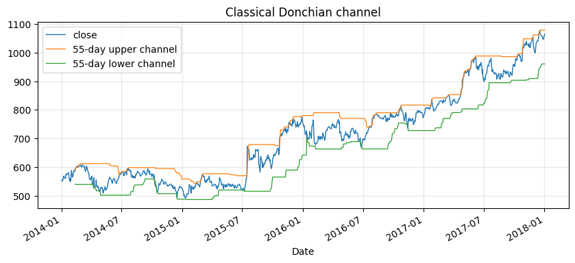
2. Classical Donchian/Turtle baselines
The baseline enters on a prior-channel breakout and exits on a shorter-channel break. The channel is shifted by one bar to avoid comparing today's close with a channel that already includes today's high.
classic_breakout_weights = make_classic_breakout_weight_grid(prices, high=high, low=low)
classic_table, classic_results = compare_weight_strategies(prices, classic_breakout_weights, fee_bps=1.0, slippage_bps=2.0)
display(classic_table[["total_return", "cagr", "sharpe", "max_drawdown", "average_turnover"]].round(4))
| total_return | cagr | sharpe | max_drawdown | average_turnover | |
|---|---|---|---|---|---|
| strategy | |||||
| classic_donchian_20_10 | 0.0530 | 0.0130 | 0.1587 | -0.1950 | 0.0407 |
| classic_turtle_55_20 | 0.0416 | 0.0102 | 0.1406 | -0.1248 | 0.0208 |
| classic_turtle_55_20_long_short | -0.2099 | -0.0572 | -0.2800 | -0.3194 | 0.0308 |
channel = donchian_channels(high, low, window=55, shift=1)
fig, ax = plt.subplots(figsize=(10, 4))
prices[ticker].plot(ax=ax, linewidth=1.0, label="close")
channel.upper[ticker].plot(ax=ax, linewidth=0.9, label="55-day upper channel")
channel.lower[ticker].plot(ax=ax, linewidth=0.9, label="55-day lower channel")
ax.set_title("Classical Donchian channel")
ax.legend()
ax.grid(True, alpha=0.3)
plt.show()
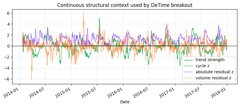
3. DeTime breakout gates
The DeTime version still needs a price breakout. It then asks four structural questions: is the trend rising, is the cycle not fighting the entry, is the residual not already overextended, and is volume participation present?
features = walkforward_decompose_ohlcv(
    ohlcv,
    method="STL",
    period="auto",
    period_candidates=(63, 126, 252),
    train_window=504,
    step=5,
    z_window=63,
)
feature_tail = build_feature_table(prices, features).tail(120)
display(feature_tail.tail(5).round(4))
feature_tail.to_csv(report_dir / "column_04_feature_table_tail.csv")
| component_stability | cycle | cycle_amplitude | cycle_position | cycle_slope | cycle_turn_up | cycle_z | realized_vol_20 | reconstruction_error | residual | residual_abs_z | residual_vol | residual_z | return_1d | season | ... | volume_cycle_turn_up | volume_cycle_z | volume_participation | volume_reconstruction_error | volume_residual | volume_residual_abs_z | volume_residual_vol | volume_residual_z | volume_selected_period | volume_shock | volume_trend | volume_trend_acceleration | volume_trend_gap | volume_trend_slope | volume_trend_strength | |
|---|---|---|---|---|---|---|---|---|---|---|---|---|---|---|---|---|---|---|---|---|---|---|---|---|---|---|---|---|---|---|---|
| GOOG | GOOG | GOOG | GOOG | GOOG | GOOG | GOOG | GOOG | GOOG | GOOG | GOOG | GOOG | GOOG | GOOG | GOOG | ... | GOOG | GOOG | GOOG | GOOG | GOOG | GOOG | GOOG | GOOG | GOOG | GOOG | GOOG | GOOG | GOOG | GOOG | GOOG | |
| Date | |||||||||||||||||||||||||||||||
| 2017-12-26 | 0.9853 | 0.0456 | 0.0438 | 1.0414 | -0.0051 | 0.0 | 0.6138 | 0.1515 | 0.0 | 0.0004 | 0.1109 | 0.0149 | 0.1109 | -0.0032 | 0.0456 | ... | 0.0 | -0.5708 | 2.0 | 0.0 | -0.2911 | 2.3259 | 0.1243 | -2.3259 | 126.0 | 2.3259 | 14.0559 | -0.0 | -0.514 | -0.0011 | -0.0031 |
| 2017-12-27 | 0.9853 | 0.0456 | 0.0438 | 1.0414 | -0.0051 | 0.0 | 0.6138 | 0.1518 | 0.0 | 0.0004 | 0.1109 | 0.0149 | 0.1109 | -0.0070 | 0.0456 | ... | 0.0 | -0.5708 | 2.0 | 0.0 | -0.2911 | 2.3259 | 0.1243 | -2.3259 | 126.0 | 2.3259 | 14.0559 | -0.0 | -0.514 | -0.0011 | -0.0031 |
| 2017-12-28 | 0.9853 | 0.0456 | 0.0438 | 1.0414 | -0.0051 | 0.0 | 0.6138 | 0.1226 | 0.0 | 0.0004 | 0.1109 | 0.0149 | 0.1109 | -0.0012 | 0.0456 | ... | 0.0 | -0.5708 | 2.0 | 0.0 | -0.2911 | 2.3259 | 0.1243 | -2.3259 | 126.0 | 2.3259 | 14.0559 | -0.0 | -0.514 | -0.0011 | -0.0031 |
| 2017-12-29 | 0.9853 | 0.0456 | 0.0438 | 1.0414 | -0.0051 | 0.0 | 0.6138 | 0.1229 | 0.0 | 0.0004 | 0.1109 | 0.0149 | 0.1109 | -0.0017 | 0.0456 | ... | 0.0 | -0.5708 | 2.0 | 0.0 | -0.2911 | 2.3259 | 0.1243 | -2.3259 | 126.0 | 2.3259 | 14.0559 | -0.0 | -0.514 | -0.0011 | -0.0031 |
| 2018-01-02 | 0.9853 | 0.0456 | 0.0438 | 1.0414 | -0.0051 | 0.0 | 0.6138 | 0.1270 | 0.0 | 0.0004 | 0.1109 | 0.0149 | 0.1109 | 0.0178 | 0.0456 | ... | 0.0 | -0.5708 | 2.0 | 0.0 | -0.2911 | 2.3259 | 0.1243 | -2.3259 | 126.0 | 2.3259 | 14.0559 | -0.0 | -0.514 | -0.0011 | -0.0031 |
5 rows × 44 columns
diagnostic = decompose_one_series(
    prices[ticker],
    method="STL",
    period="auto",
    period_candidates=(63, 126, 252),
    z_window=63,
    transform="log",
)
volume_diagnostic = decompose_one_series(
    ohlcv["Volume"][ticker],
    method="STL",
    period=int(diagnostic.attrs.get("period", 126)),
    z_window=63,
    transform="log1p",
)

fig, ax = plt.subplots(figsize=(10, 3.8))
diagnostic["trend_strength"].plot(ax=ax, linewidth=1.0, color="#0f766e", label="trend strength")
diagnostic["cycle_z"].plot(ax=ax, linewidth=0.9, color="#16a34a", label="cycle z")
diagnostic["residual_abs_z"].plot(ax=ax, linewidth=0.9, color="#7c3aed", alpha=0.85, label="absolute residual z")
volume_diagnostic["residual_z"].plot(ax=ax, linewidth=0.8, color="#f97316", alpha=0.75, label="volume residual z")
ax.axhline(0, color="black", linewidth=0.8)
ax.set_title("Continuous structural context used by DeTime breakout")
ax.legend()
ax.grid(True, alpha=0.3)
plt.show()
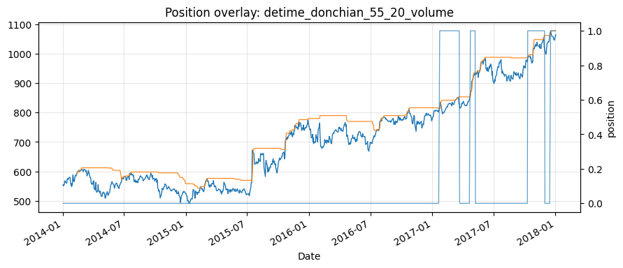
4. DeTime breakout results
The comparison is a simple research backtest showing how the signal is constructed and audited.
detime_breakout_weights = make_detime_breakout_weight_grid(prices, features, high=high, low=low)
detime_table, detime_results = compare_weight_strategies(prices, detime_breakout_weights, fee_bps=1.0, slippage_bps=2.0)
display(detime_table[["total_return", "cagr", "sharpe", "max_drawdown", "average_turnover"]].round(4))
| total_return | cagr | sharpe | max_drawdown | average_turnover | |
|---|---|---|---|---|---|
| strategy | |||||
| detime_donchian_55_20_volume | 0.0863 | 0.0209 | 0.4521 | -0.0697 | 0.0069 |
| detime_turtle_55_20 | 0.0863 | 0.0209 | 0.4521 | -0.0697 | 0.0069 |
| detime_donchian_20_10_volume | -0.1479 | -0.0392 | -0.5046 | -0.1946 | 0.0248 |
classical = run_classical_breakout_baselines(prices, high=high, low=low, fee_bps=1.0, slippage_bps=2.0)
detime = run_detime_breakout_baselines(prices, features, high=high, low=low, fee_bps=1.0, slippage_bps=2.0)
comparison = compare_classical_and_detime(classical, detime)
display(comparison[["strategy_group", "cagr", "sharpe", "max_drawdown", "average_turnover", "hit_rate"]].round(4))
comparison.to_csv(report_dir / "column_04_strategy_comparison.csv")
write_run_audit(report_dir, data_manifest=manifest, audit=audit, strategy_stats=comparison, prefix="column_04")
manifest_path = write_run_manifest(
    report_dir / "column_04_run_manifest.json",
    command="notebook:04_turtle_donchian_breakout_volume_confirmation",
    dataset="bundled_real_GOOG",
    strategies=list(comparison.index),
    result_file=str(report_dir / "column_04_strategy_comparison.csv"),
)
manifest_path.as_posix()
| strategy_group | cagr | sharpe | max_drawdown | average_turnover | hit_rate | |
|---|---|---|---|---|---|---|
| strategy | ||||||
| detime_donchian_55_20_volume | detime | 0.0209 | 0.4521 | -0.0697 | 0.0069 | 0.0526 |
| detime_turtle_55_20 | detime | 0.0209 | 0.4521 | -0.0697 | 0.0069 | 0.0526 |
| classic_donchian_20_10 | classical | 0.0130 | 0.1587 | -0.1950 | 0.0407 | 0.2351 |
| classic_turtle_55_20 | classical | 0.0102 | 0.1406 | -0.1248 | 0.0208 | 0.1925 |
| classic_turtle_55_20_long_short | classical | -0.0572 | -0.2800 | -0.3194 | 0.0308 | 0.2569 |
| detime_donchian_20_10_volume | detime | -0.0392 | -0.5046 | -0.1946 | 0.0248 | 0.0734 |
'examples/quant_trading/reports/column_04_run_manifest.json'
chosen = "detime_donchian_55_20_volume"
fig, ax1 = plt.subplots(figsize=(10, 4))
prices[ticker].plot(ax=ax1, linewidth=1.0, label="close")
channel.upper[ticker].plot(ax=ax1, linewidth=0.8, label="55-day upper")
ax1.set_title(f"Position overlay: {chosen}")
ax2 = ax1.twinx()
detime_breakout_weights[chosen][ticker].plot(ax=ax2, linewidth=0.9, alpha=0.7, label="position")
ax2.set_ylabel("position")
ax1.grid(True, alpha=0.3)
plt.show()
Takeaway
A channel breakout is a price event. A tradable breakout also needs context. DeTime supplies that context explicitly: trend estimates direction, cycle estimates whether the entry is fighting a local oscillation, residual caps overextension, and decomposed volume distinguishes participation from ordinary noise.