Wavelet decomposition
Wavelet decomposition
| Property | Value |
|---|---|
| Method | WAVELET |
| Input mode | univariate |
| Trend shape | (96,) |
| Notebook execution | ran |
| Reconstruction RMSE | 0.00000000 |
Notebook example metric: root mean square of input - (trend + season + residual) over all samples and channels. This checks additive bookkeeping; it is not a forecast error or a component-recovery score. The separate teaching input and intermediate arrays for the animation are linked below.
How it works
Method maturity: stable. Implementation: wrapper.
A discrete wavelet transform separates scales through paired low-pass and high-pass filters. DeTime reconstructs selected coefficient blocks onto the original sample grid.
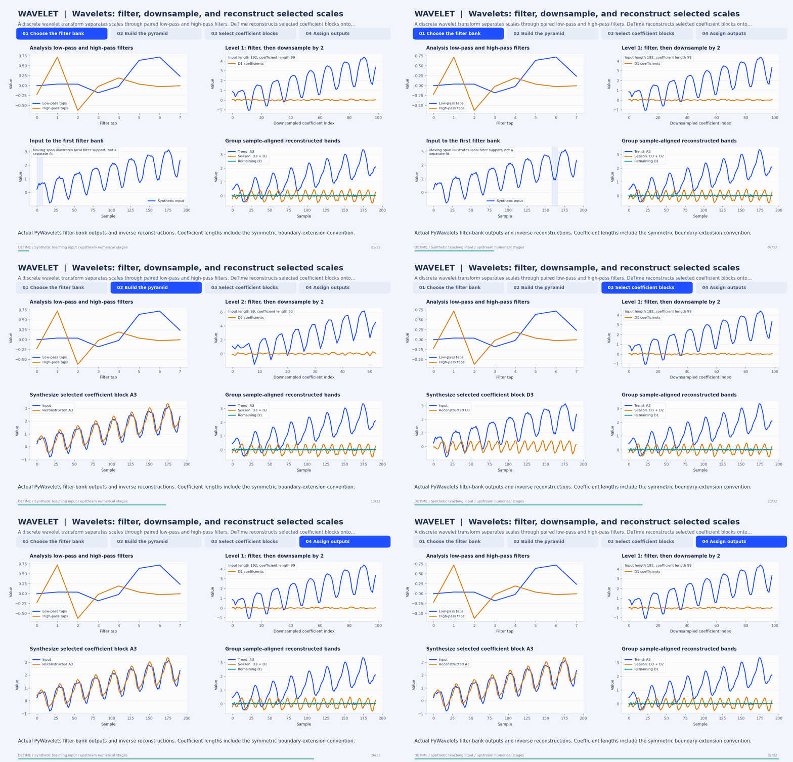
Deterministic synthetic teaching signal; not a benchmark.
Open GIF · Static PNG · Source arrays (NPZ) · Trace metadata
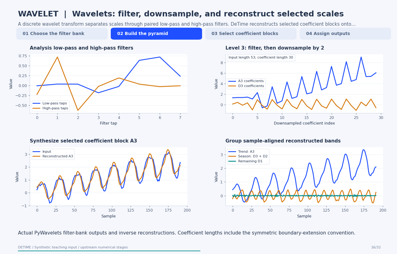
Follow the four steps
1. Choose the filter bank
The wavelet fixes the analysis and synthesis filters; this trace uses db4.
2. Build the pyramid
Low-pass and high-pass filtering are followed by decimation; repeat on the approximation.
3. Select coefficient blocks
Retain a block, zero the others, and apply the inverse transform to obtain a sample-aligned contribution.
4. Assign outputs
This example assigns A3 to trend and D3+D2 to season; the remainder is input minus those outputs.
Parameters that change the result
| Parameter | Effect on the computation |
|---|---|
wavelet |
Controls filters and their support; db4 has eight analysis taps. |
level |
Controls pyramid depth; the example uses three levels. |
trend_levels / season_levels |
Indexes the wavedec list [A3,D3,D2,D1] here, not ascending physical scales. |
Boundary convention |
The current wrapper uses PyWavelets' default symmetric mode. |
What this animation computes
Computed with PyWavelets 1.10.0; inverse band reconstructions call the current DeTime helper. Moving filter support is a labeled illustration; coefficient values are actual library outputs.
Interpretation
- Wavelet detail coefficients are decimated and should not be mistaken for sample-aligned output curves.
- Assigning scales to trend or season is an application choice; the transform does not identify physical mechanisms.
- The animation uses a safe fixed depth; excessive levels make boundary effects dominate.
Try the method
Use this configuration with DecompositionConfig and decompose. The animation generator supplies the teaching input and records intermediate arrays.
{
  "method": "WAVELET",
  "params": {
    "wavelet": "db4",
    "level": 3,
    "trend_levels": [
      0
    ],
    "season_levels": [
      1,
      2
    ]
  }
}
See the configuration reference for the full interface and optional dependencies.
Sources and reproduction
- PyWavelets discrete transform
- Inverse transform and partial reconstruction
- Signal-extension modes
- DeTime implementation:
src/detime/methods/wavelet.py
Regenerate this animation with python scripts/generate_method_animations.py --methods WAVELET.
The reproduction guide explains the environment,
numerical checks, coverage manifest, and how to inspect the stored arrays.
Code
case = CASES["WAVELET"]
run_gallery_case("WAVELET")
Output
WAVELET: Wavelet-based decomposition exposed through the common output contract.
status: ran
input mode: univariate
trend shape: (96,)
backend: python
reconstruction RMSE: 0.00000000
Decomposition Plot
